7.9. Hypothesis Testing of a Single Proportion

Hypothesis testing of a single proportion is a statistical method used to determine if the proportion of a certain attribute in a population significantly differs from a hypothesized proportion. This type of test is commonly used in various fields, including social sciences, medicine, and quality control.

For hypothesis testing involving a population proportion (\(p\)), the null and alternative hypotheses are established as follows:

7.9.1. Null Hypothesis (\(H_0\))

The null hypothesis can take one of three forms, depending on the context of the test:

1. \(H_0: p = p_0\): The population proportion is equal to a specific value, \(p_0\).

2. \(H_0: p \geq p_0\): The population proportion is greater than or equal to a certain value, \(p_0\).

3. \(H_0: p \leq p_0\): The population proportion is less than or equal to a certain value, \(p_0\).

Here, \(p_0\) represents the hypothesized population proportion that serves as the reference point for the test.

7.9.2. Alternative Hypothesis (\(H_a\))

The alternative hypothesis represents the hypothesis that is tested against the null hypothesis. It can be one of the following, depending on the research question:

1. Two-Tailed Test:

   (7.16)\[\begin{equation} H_a: p \neq p_0 \end{equation}\]

   This test checks if the population proportion is different from \(p_0\), either higher or lower.

2. Left-Tailed Test:

   (7.17)\[\begin{equation} H_a: p < p_0 \end{equation}\]

   This test checks if the population proportion is less than \(p_0\).

3. Right-Tailed Test:

   (7.18)\[\begin{equation} H_a: p > p_0 \end{equation}\]

   This test checks if the population proportion is greater than \(p_0\).

The choice of the alternative hypothesis depends on the specific objective of the study. Aligning the hypothesis test with the research question ensures accurate and meaningful results.

A summary of the null and alternative hypotheses for population proportion tests is provided in Table 7.4:

Table 7.4 Null and alternative hypotheses for population proportion tests.

Test Type	Null Hypothesis (\(H_0\))	Alternative Hypothesis (\(H_a\))
Two-Tailed Test	\(p = p_0\)	\(p \neq p_0\)
Left-Tailed Test	\(p = p_0\) or \(p \geq p_0\)	\(p < p_0\)
Right-Tailed Test	\(p = p_0\) or \(p \leq p_0\)	\(p > p_0\)

7.9.3. Steps in Hypothesis Testing

0. Assumptions

   • Random Sampling: The sample should be randomly selected from the population.

   • Sample Size: The sample size should be large enough to ensure the normality of the sampling distribution of the proportion. A common rule of thumb is that both \(np_0\) and \(n(1 - p_0)\) should be at least 5.

1. Select the Significance Level (\(\alpha\))

   • The significance level, commonly set at 0.05, defines the probability of rejecting the null hypothesis when it is true (Type I error).

2. Calculate the Test Statistic

   • The test statistic for a single proportion is calculated using the formula:

     (7.19)\[\begin{equation} z = \dfrac{\hat{p} - p_0}{\sqrt{\dfrac{p_0 (1 - p_0)}{n}}} \end{equation}\]

     where \(\hat{p}\) is the sample proportion, \(p_0\) is the hypothesized proportion, and \(n\) is the sample size.

3. Determine the Critical Value or P-value

   • The critical value is based on the chosen significance level and the type of test (one-tailed or two-tailed). Alternatively, the p-value, which represents the probability of obtaining a test statistic as extreme as the one observed, under the assumption that the null hypothesis is true, can be calculated.

4. Make a Decision

   • Compare the test statistic to the critical value or compare the p-value to the significance level:

     • If the test statistic exceeds the critical value (or the p-value is less than \(\alpha\)), reject the null hypothesis.

     • Otherwise, fail to reject the null hypothesis.

Algorithm 7.3 (Hypothesis Tests for One Population Proportion)

Objective: To conduct a hypothesis test for a population proportion (\(p\)).

Prerequisites:

1. A simple random sample is obtained.

2. The sample size is large enough to ensure the normality of the sampling distribution of the proportion. A common rule of thumb is that both \(np_0\) and \(n(1 - p_0)\) should be at least 5.

Method:

1. Define the Significance Level: Choose the significance level (\(\alpha\)).

2. State the Hypotheses:

   • Two-Tailed Test:

     • Null Hypothesis: \(H_0: p = p_{0}\)

     • Alternative Hypothesis: \(H_a: p \neq p_{0}\)

   • Left-Tailed Test:

     • Null Hypothesis: \(H_0: p \geq p_{0}\)

     • Alternative Hypothesis: \(H_a: p < p_{0}\)

   • Right-Tailed Test:

     • Null Hypothesis: \(H_0: p \leq p_{0}\)

     • Alternative Hypothesis: \(H_a: p > p_{0}\)

3. Calculate the Test Statistic: Use the formula:

   (7.20)\[\begin{equation} z = \dfrac{\hat{p} - p_{0}}{\sqrt{\dfrac{p_{0} (1 - p_{0})}{n}}} \end{equation}\]

   where \(\hat{p}\) is the sample proportion, \(p_{0}\) is the hypothesized proportion, and \(n\) is the sample size.

4. Determine Critical Value(s) or P-value:

   • For two-tailed tests: \(\pm z_{\alpha/2}\)

   • For left-tailed tests: \(-z_{\alpha}\)

   • For right-tailed tests: \(z_{\alpha}\)

   Alternatively, calculate the p-value using the test statistic.

5. Decision Rule:

   • Critical-Value Approach:

     • If the test statistic falls within the rejection region, reject \(H_0\); otherwise, do not reject \(H_0\).

   • P-value Approach:

     • Reject \(H_0\) if \(p \leq \alpha\); otherwise, do not reject \(H_0\).

This algorithm outlines the steps to perform a hypothesis test for a population proportion. It ensures appropriate handling of the sample data to draw valid conclusions about the population proportion.

Example 7.41

A researcher claims that the proportion of people who prefer online shopping over in-store shopping is more than 60%. To test this claim, a random sample of 150 people was surveyed, and 100 of them preferred online shopping.

At the 5% significance level, do the data provide sufficient evidence to conclude that the proportion of people who prefer online shopping is more than 60%?

Solution:

Hypothesis Test:

• Null Hypothesis (\(H_0\)): \(p \leq 0.60\)

• Alternative Hypothesis (\(H_a\)): \(p > 0.60\)

Sample Statistics:

• \(n = 150\)

• \(\hat{p} = \frac{100}{150} = 0.67\)

Significance Level: \(\alpha = 0.05\)

Test Statistic:

\[\begin{equation*} z = \dfrac{\hat{p} - p_0}{\sqrt{\dfrac{p_0 (1 - p_0)}{n}}} = \dfrac{0.6667 - 0.60}{\sqrt{\dfrac{0.60 (1 - 0.60)}{150}}} \approx 1.667 \end{equation*}\]

Critical-Value Approach:

• Critical value: \(z_{\alpha} = z_{0.05} \approx 1.645\)

Since \(\text{Test Statistic} = 1.667 > z_{0.05} = 1.645\), reject \(H_0\).

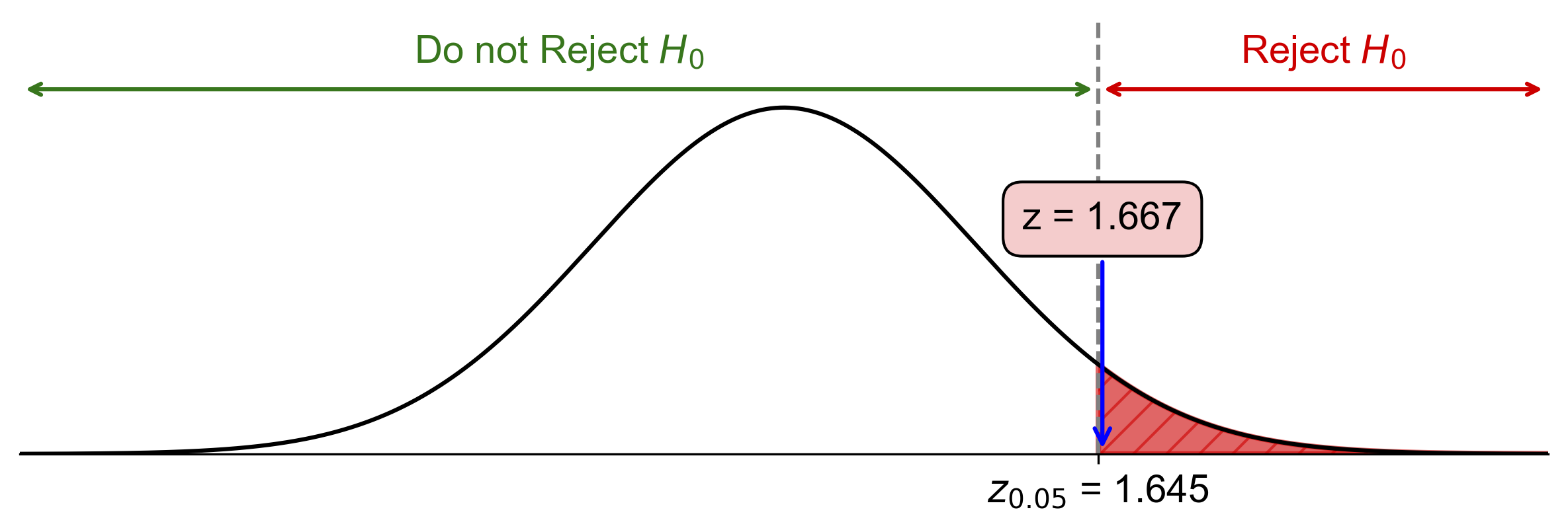
Fig. 7.52 Critical-value approach illustrating the rejection region and test statistic for Example 7.41.

At the 5% significance level, the data provide sufficient evidence to conclude that the proportion of people who prefer online shopping is more than 60%.

P-Value Approach:

• P-value: \(P(Z > 1.667) \approx 0.0478\)

Since \(\text{P-value} = 0.0478 < \alpha = 0.05\), reject \(H_0\).

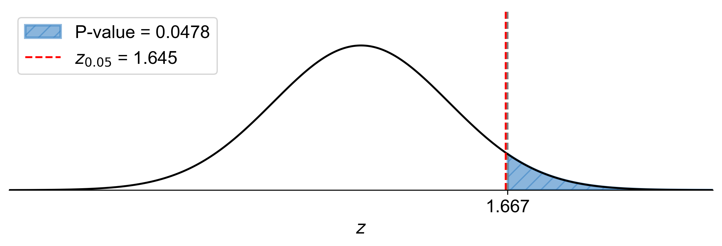
Fig. 7.53 P-value approach demonstrating the significance of the test statistic in relation to the null hypothesis for Example 7.41.

At the 5% significance level, the data provide sufficient evidence to conclude that the proportion of people who prefer online shopping is more than 60%.

Example 7.42

A company claims that at least 70% of its customers are satisfied with their service. To test this claim, a random sample of 200 customers was surveyed, and 130 of them reported being satisfied.

At the 5% significance level, do the data provide sufficient evidence to conclude that the proportion of satisfied customers is less than 70%?

Solution:

Hypothesis Test:

• Null Hypothesis (\(H_0\)): \(p \geq 0.70\)

• Alternative Hypothesis (\(H_a\)): \(p < 0.70\)

Sample Statistics:

• \(n = 200\)

• \(\hat{p} = \frac{130}{200} = 0.65\)

Significance Level: \(\alpha = 0.05\)

Test Statistic:

\[\begin{equation*} z = \dfrac{\hat{p} - p_0}{\sqrt{\dfrac{p_0 (1 - p_0)}{n}}} = \dfrac{0.65 - 0.70}{\sqrt{\dfrac{0.70 (1 - 0.70)}{200}}} \approx -1.543 \end{equation*}\]

Critical-Value Approach:

• Critical value: \(z_{\alpha} = z_{0.05} \approx -1.645\)

Since \(\text{Test Statistic} = -1.54 > z_{0.05} = -1.645\), fail to reject \(H_0\).

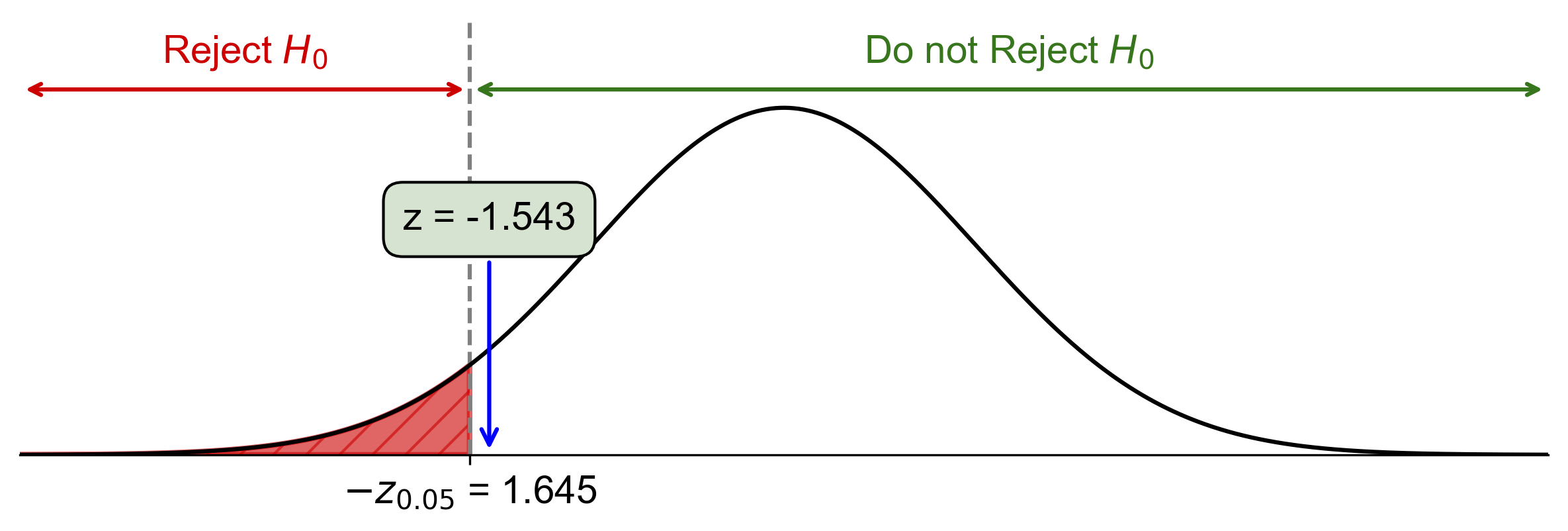
Fig. 7.54 Critical-value approach illustrating the rejection region and test statistic for Example 7.42.

At the 5% significance level, the data do not provide sufficient evidence to conclude that the proportion of satisfied customers is less than 70%.

P-Value Approach:

• P-value: \(P(Z < -1.54) \approx 0.0614\)

Since \(\text{P-value} = 0.0614 > \alpha = 0.05\), fail to reject \(H_0\).

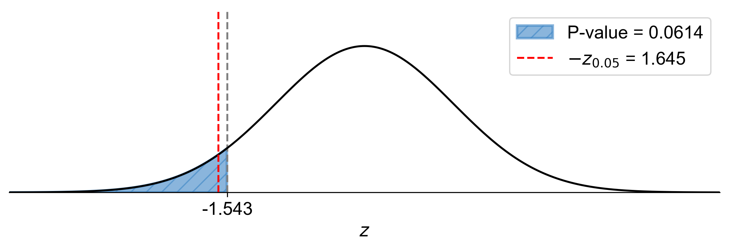
Fig. 7.55 P-value approach demonstrating the significance of the test statistic in relation to the null hypothesis for Example 7.42.

At the 5% significance level, the data do not provide sufficient evidence to conclude that the proportion of satisfied customers is less than 70%.

Example 7.43

A researcher claims that the proportion of people who prefer electric cars over gasoline cars is more than 30%. To test this claim, a random sample of 200 people was surveyed, and 75 of them preferred electric cars.

At the 5% significance level, do the data provide sufficient evidence to conclude that the proportion of people who prefer electric cars is more than 30%?

Solution:

Hypothesis Test:

• Null Hypothesis (\(H_0\)): \(p \leq 0.30\)

• Alternative Hypothesis (\(H_a\)): \(p > 0.30\)

Sample Statistics:

• \(n = 200\)

• \(\hat{p} = \dfrac{75}{200} = 0.375\)

Significance Level: \(\alpha = 0.05\)

Test Statistic:

\[\begin{equation*} z = \dfrac{\hat{p} - p_0}{\sqrt{\dfrac{p_0 (1 - p_0)}{n}}} = \dfrac{0.375 - 0.30}{\sqrt{\dfrac{0.30 (1 - 0.30)}{200}}} \approx 2.315 \end{equation*}\]

Critical-Value Approach:

• Critical value: \(z_{\alpha} = z_{0.05} \approx 1.645\)

Since \(\text{Test Statistic} = 2.315 > z_{0.05} = 1.645\), reject \(H_0\).

At the 5% significance level, the data provide sufficient evidence to conclude that the proportion of people who prefer electric cars is more than 30%.

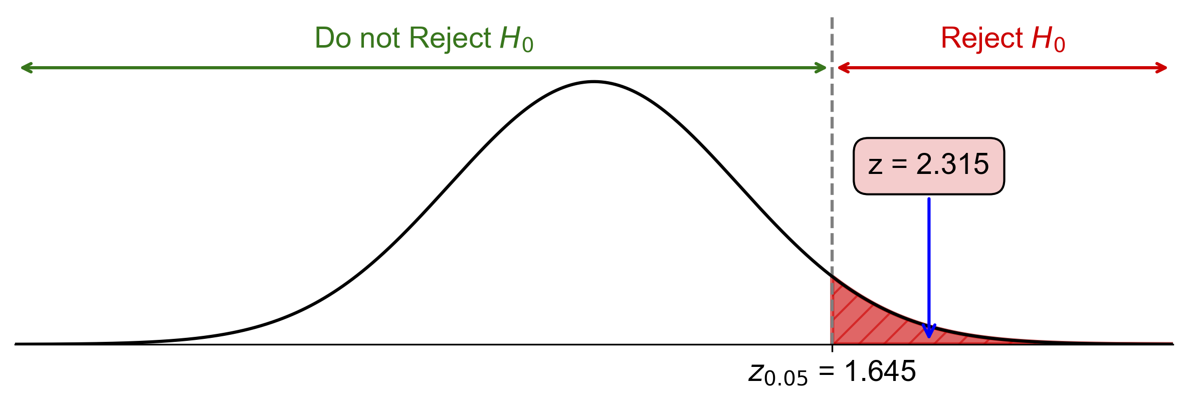
Fig. 7.56 Critical-value approach illustrating the rejection region and test statistic for Example 7.43.

P-Value Approach:

• P-value: \(P(Z > 2.315) \approx 0.0103\)

Since \(\text{P-value} = 0.0103 < \alpha = 0.05\), reject \(H_0\).

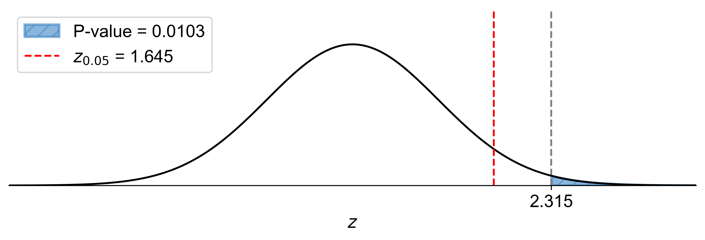
Fig. 7.57 P-value approach demonstrating the significance of the test statistic in relation to the null hypothesis for Example 7.43.

At the 5% significance level, the data provide sufficient evidence to conclude that the proportion of people who prefer electric cars is more than 30%.

Example 7.44

A researcher claims that the proportion of people who exercise regularly is more than 30%. To test this claim, a random sample of 200 people was surveyed, and 70 of them reported exercising regularly.

At the 1% significance level, do the data provide sufficient evidence to conclude that the proportion of people who exercise regularly is more than 30%?

Solution:

Hypothesis Test:

• Null Hypothesis (\(H_0\)): \(p \leq 0.30\)

• Alternative Hypothesis (\(H_a\)): \(p > 0.30\)

Sample Statistics:

• \(n = 200\)

• \(\hat{p} = \frac{70}{200} = 0.35\)

Significance Level: \(\alpha = 0.05\)

Test Statistic:

\[\begin{equation*} z = \dfrac{\hat{p} - p_0}{\sqrt{\dfrac{p_0 (1 - p_0)}{n}}} = \dfrac{0.35 - 0.30}{\sqrt{\dfrac{0.30 (1 - 0.30)}{200}}} \approx 1.543 \end{equation*}\]

Critical-Value Approach:

• Critical value: \(z_{\alpha} = z_{0.01} \approx 2.326\)

Since \(\text{Test Statistic} = 1.543 < z_{0.01} = 2.326\), fail to reject \(H_0\).

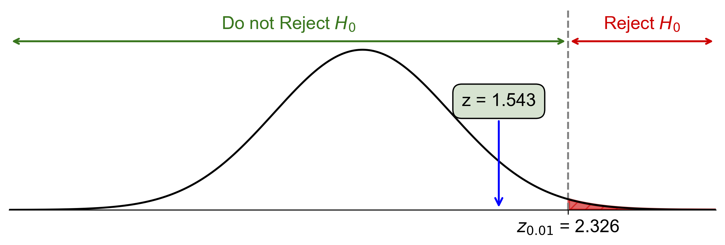
Fig. 7.58 Critical-value approach illustrating the rejection region and test statistic for Example 7.44.

At the 1% significance level, the data do not provide sufficient evidence to conclude that the proportion of people who exercise regularly is more than 30%.

P-Value Approach:

• P-value: \(P(Z > 1.543) \approx 0.0614\)

Since \(\text{P-value} = 0.0614 > \alpha = 0.01\), fail to reject \(H_0\).

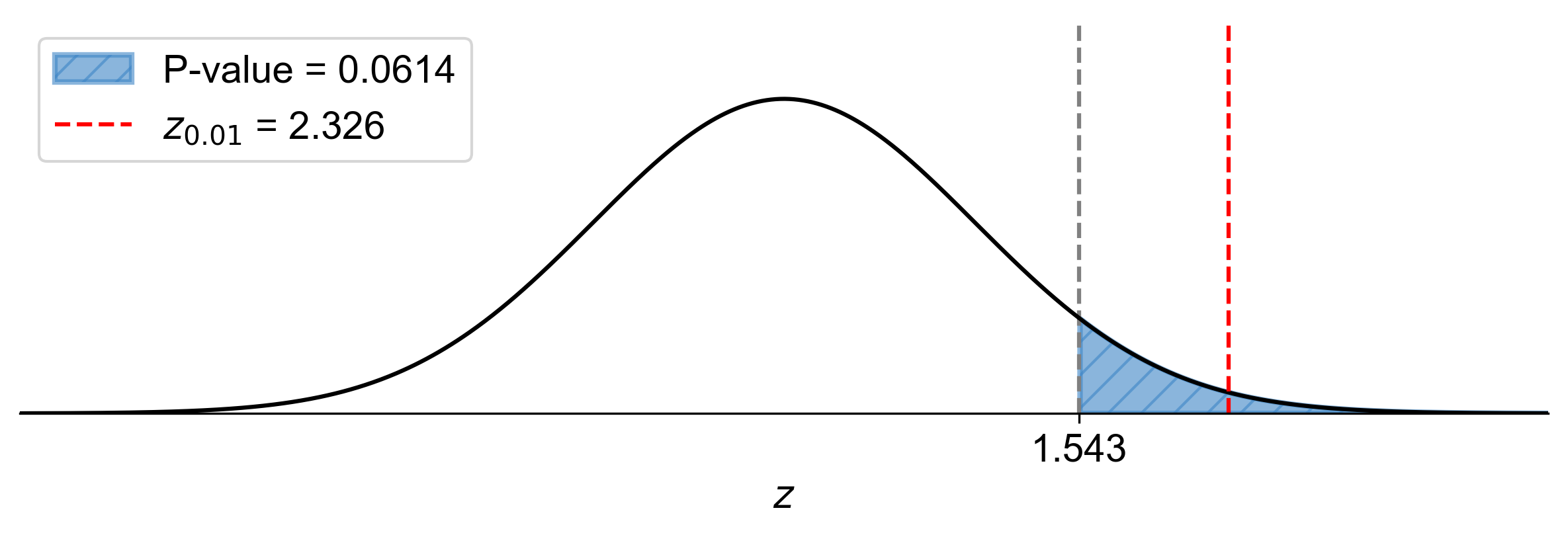
Fig. 7.59 P-value approach demonstrating the significance of the test statistic in relation to the null hypothesis for Example 7.44.

At the 1% significance level, the data do not provide sufficient evidence to conclude that the proportion of people who exercise regularly is more than 30%.

Example 7.45

A researcher claims that the proportion of people who prefer tea over coffee is different from 40%. To test this claim, a random sample of 250 people was surveyed, and 110 of them preferred tea.

At the 5% significance level, do the data provide sufficient evidence to conclude that the proportion of people who prefer tea is different from 40%?

Solution:

Hypothesis Test:

• Null Hypothesis (\(H_0\)): \(p = 0.40\)

• Alternative Hypothesis (\(H_a\)): \(p \neq 0.40\)

Sample Statistics:

• \(n = 250\)

• \(\hat{p} = \frac{110}{250} = 0.44\)

Significance Level: \(\alpha = 0.05\)

Test Statistic:

\[\begin{equation*} z = \dfrac{\hat{p} - p_0}{\sqrt{\dfrac{p_0 (1 - p_0)}{n}}} = \dfrac{0.44 - 0.40}{\sqrt{\dfrac{0.40 (1 - 0.40)}{250}}} \approx 1.291 \end{equation*}\]

Critical-Value Approach:

• Critical value: \(z_{\alpha/2} = z_{0.025} \approx 1.96\)

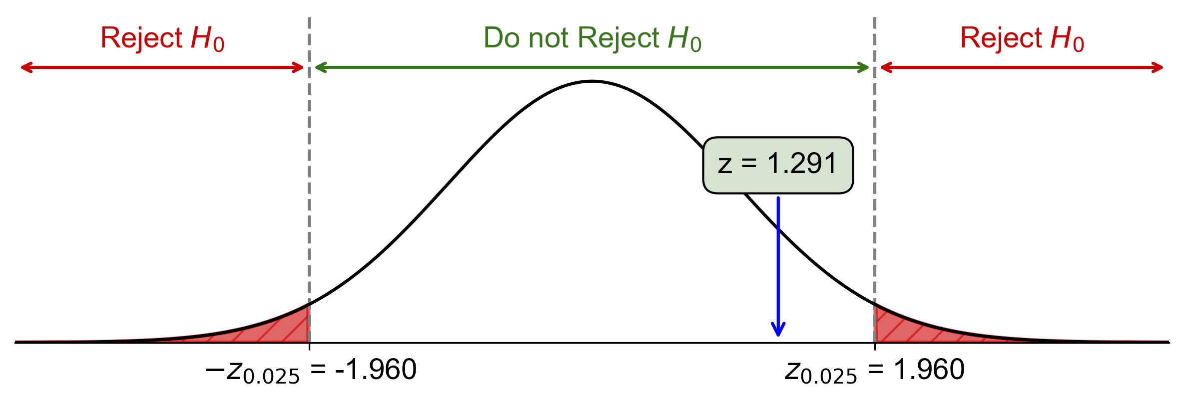
Fig. 7.60 Critical-value approach illustrating the rejection region and test statistic for Example 7.45.

Since \(\text{Test Statistic} = 1.291 < z_{0.025} = 1.96\), fail to reject \(H_0\).

At the 5% significance level, the data do not provide sufficient evidence to conclude that the proportion of people who prefer tea is different from 40%. P-Value Approach:

• P-value: \(2 \times P(Z > 1.291) \approx 0.1967\)

Since \(\text{P-value} = 0.1967 > \alpha = 0.05\), fail to reject \(H_0\).

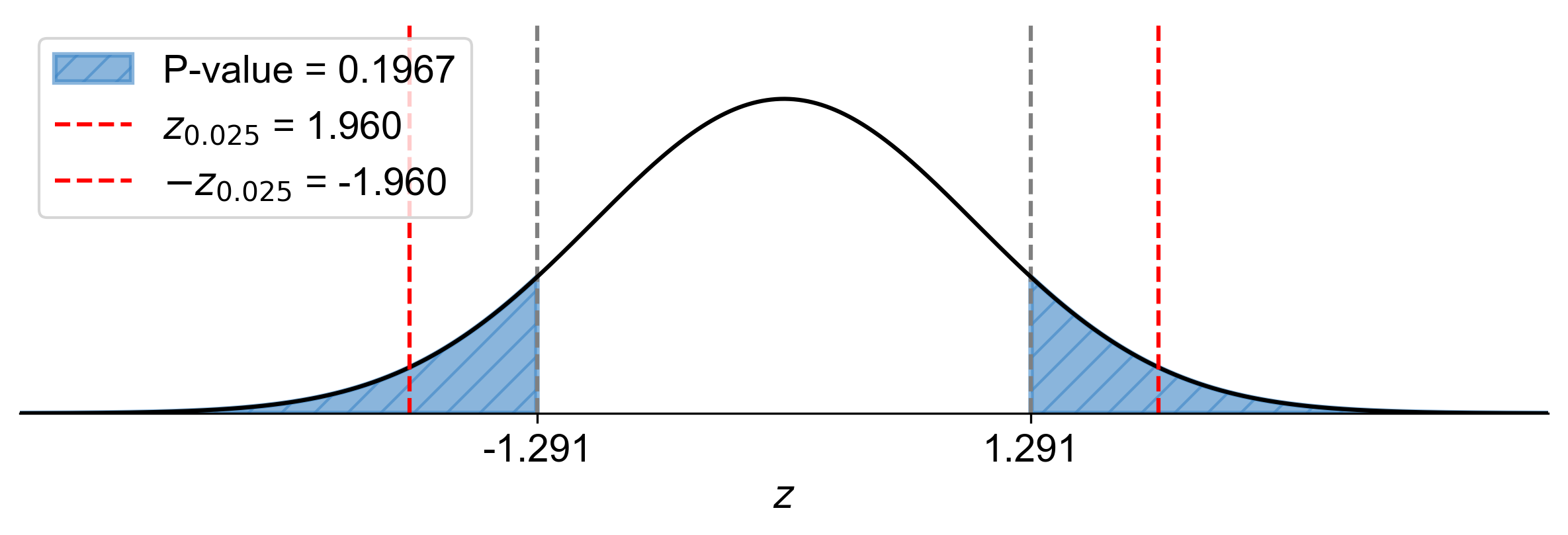
Fig. 7.61 P-value approach demonstrating the significance of the test statistic in relation to the null hypothesis for Example 7.45.

At the 5% significance level, the data do not provide sufficient evidence to conclude that the proportion of people who prefer tea is different from 40%.

Example 7.46

A researcher claims that the proportion of people who use public transportation is different from 25%. To test this claim, a random sample of 300 people was surveyed, and 90 of them reported using public transportation.

At the 1% significance level, do the data provide sufficient evidence to conclude that the proportion of people who use public transportation is different from 25%?

Solution:

Hypothesis Test:

• Null Hypothesis (\(H_0\)): \(p = 0.25\)

• Alternative Hypothesis (\(H_a\)): \(p \neq 0.25\)

Sample Statistics:

• \(n = 300\)

• \(\hat{p} = \frac{90}{300} = 0.30\)

Significance Level: \(\alpha = 0.05\)

Test Statistic:

\[\begin{equation*} z = \dfrac{\hat{p} - p_0}{\sqrt{\dfrac{p_0 (1 - p_0)}{n}}} = \dfrac{0.30 - 0.25}{\sqrt{\dfrac{0.25 (1 - 0.25)}{300}}} \approx 2.00 \end{equation*}\]

Critical-Value Approach:

• Critical value: \(z_{\alpha/2} = z_{0.025} \approx 2.576\)

Since \(\text{Test Statistic} = 2.00 < z_{0.025} = 2.576\), fail to reject \(H_0\).

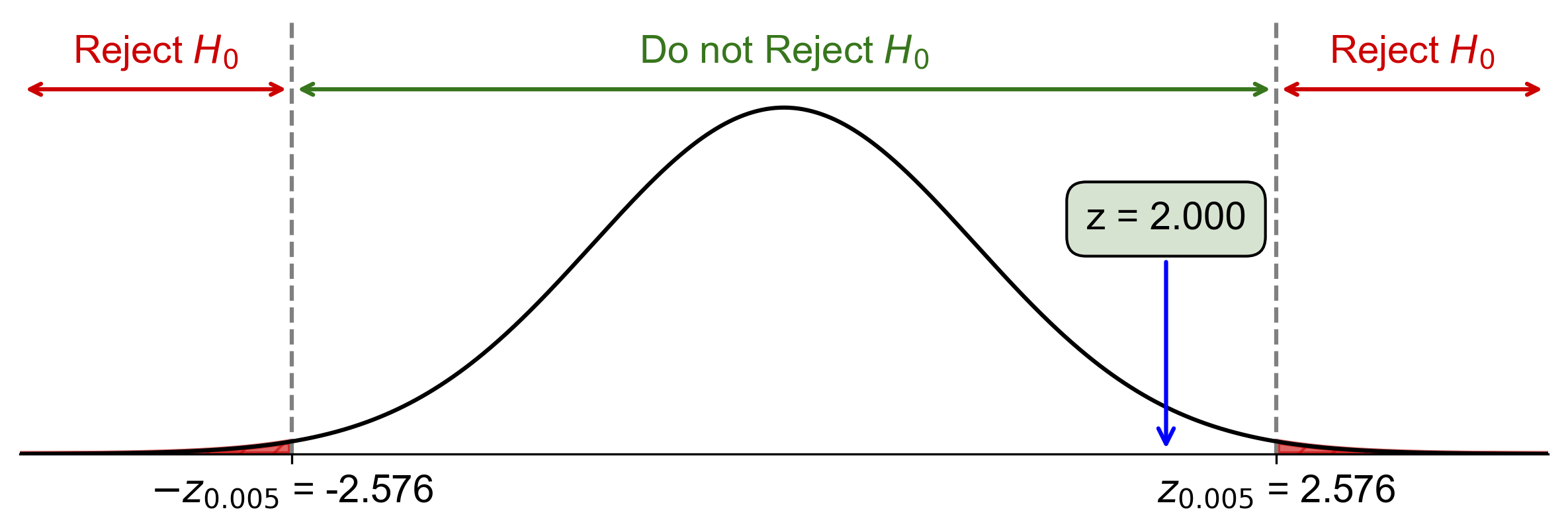
Fig. 7.62 Critical-value approach illustrating the rejection region and test statistic for Example 7.46.

At the 1% significance level, the data do not provide sufficient evidence to conclude that the proportion of people who use public transportation is different from 25%. P-Value Approach:

• P-value: \(2 \times P(Z > 2.00) \approx 0.0455\)

Since \(\text{P-value} = 0.0455 > \alpha = 0.05\), fail to reject \(H_0\).

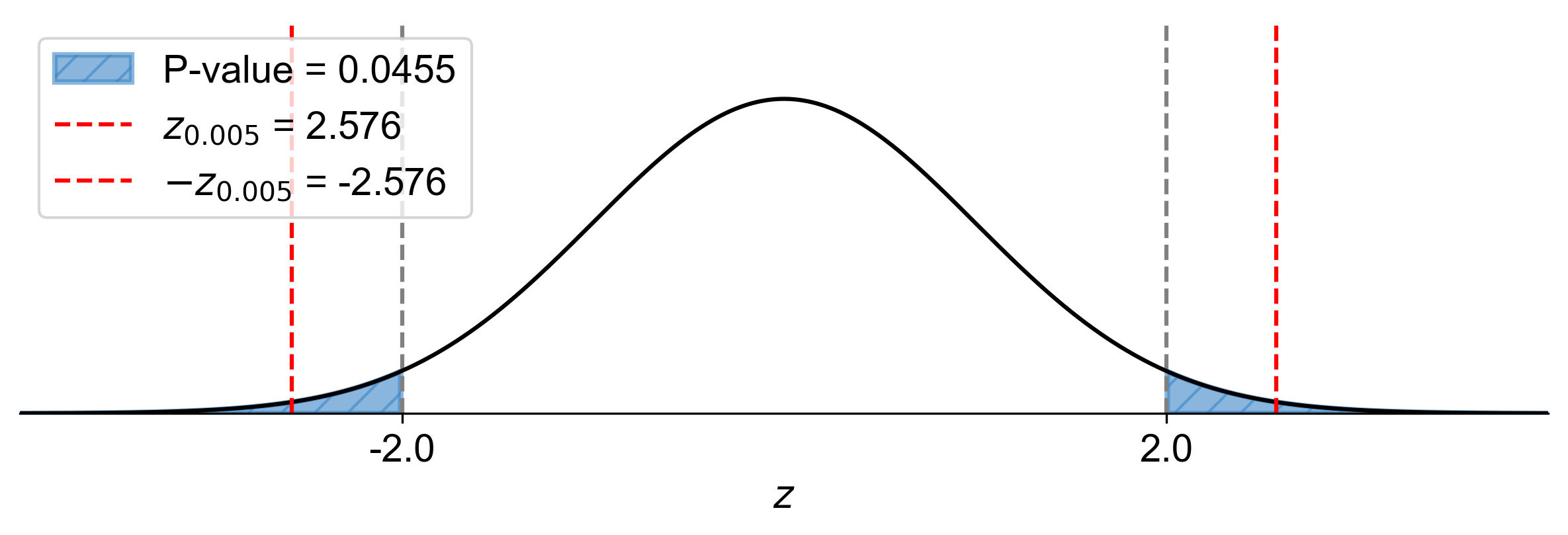
Fig. 7.63 P-value approach demonstrating the significance of the test statistic in relation to the null hypothesis for Example 7.46.

At the 1% significance level, the data do not provide sufficient evidence to conclude that the proportion of people who use public transportation is different from 25%.