8.1. Normal Distribution Table#
In Section 5.4 section, we explored how to use a normal distribution table. For convenience, both the positive and negative sides of the z-score table are available here.
Brief Instructions for Using Standard Normal Distribution Table
Find the z-score: Determine the z-score for your data point, which is the number of standard deviations away from the mean.
Locate the z-score on the table: The leftmost column represents the first two digits and the top row represents the second decimal place of the z-score.
Interpret the table value: The value at the intersection is the cumulative probability up to that z-score.
Example: Suppose you have a z-score of 1.85. You would find the row for 1.8 and the column for 0.05. The intersection value is 0.9671, which means there’s a 96.71% probability that a standard normal variable will be less than or equal to 1.85.
8.1.1. Positive Side of z-score Table#

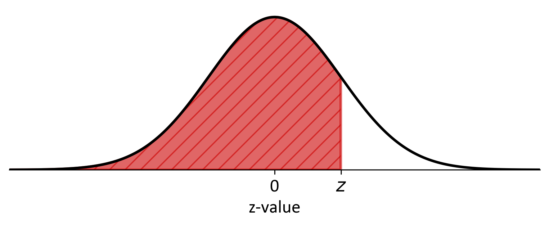
Fig. 8.1 Normal Distribution curve illustrating a positive z-score#
The standard normal distribution table, commonly known as a Z-table, is a fundamental tool in statistics for determining probabilities associated with specific z-scores. Understanding its structure is crucial for effective use:
Vertical Axis (z): This column lists z-scores, representing the number of standard deviations a data point is from the mean. Z-scores are typically presented to two decimal places. The first decimal place is found in the leftmost column, while the second decimal place is located in the top row. For instance, to locate a z-score of 1.2, you would refer to the row beginning with 1.2.
Horizontal Axis (Top Row): This row denotes the second decimal place of the z-score. To find the probability for a specific z-score, you combine the values from both axes. For example, for a z-score of 1.23, you would first identify the 1.2 row, then move across to the 0.03 column.
The intersection point of the selected row and column provides the area under the curve to the left of the z-score. For example, a z-score of 1.23 corresponds to a table value of approximately 0.8907, indicating that roughly 89.07% of the data in a standard normal distribution falls to the left of this z-score.
It’s important to note that the table values represent cumulative probabilities from negative infinity up to the given z-score. To find the area to the right of a z-score, subtract the table value from 1. For instance, the area to the right of a z-score of 1.23 is calculated as 1 - 0.8907 = 0.1093, or 10.93%.
| 0.0 | 0.01 | 0.02 | 0.03 | 0.04 | 0.05 | 0.06 | 0.07 | 0.08 | 0.09 | |
|---|---|---|---|---|---|---|---|---|---|---|
| z | ||||||||||
|
Loading ITables v2.2.3 from the init_notebook_mode cell...
(need help?) |
8.1.2. Negative Side of z-score Table#

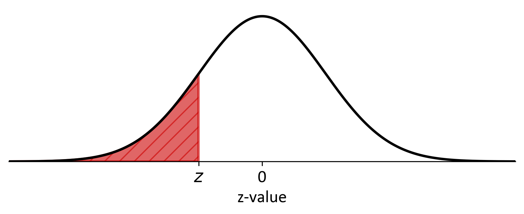
Fig. 8.2 Normal Distribution curve illustrating a negative z-score#
The negative side of the z-table is crucial for interpreting z-scores below the mean in a standard normal distribution. Understanding this aspect enhances your ability to analyze data across the entire distribution spectrum:
Negative Z-scores: These scores represent values below the mean (which is zero in a standard normal distribution). They indicate data points that fall to the left of the mean on the distribution curve.
Cumulative Probability: For negative z-scores, the table values represent the area under the curve from negative infinity up to the given z-score. For instance, a z-score of -1.23 corresponds to the cumulative probability of all values from the far left of the distribution up to -1.23 standard deviations from the mean.
Symmetry Principle: The standard normal distribution is symmetrical, making the negative side a mirror image of the positive side. This symmetry allows for a convenient calculation method: the probability associated with a negative z-score equals 1 minus the probability of its positive counterpart.
To use the z-table for negative scores:
Find the corresponding positive z-score in the table.
Subtract the table value from 1 to get the cumulative probability for the negative z-score.
For example, with a z-score of -1.23:
Look up 1.23 in the z-table (approximately 0.8907).
Calculate: 1 - 0.8907 = 0.1093.
This result indicates that about 10.93% of the data in a standard normal distribution falls below a z-score of -1.23.
| 0.09 | 0.08 | 0.07 | 0.06 | 0.05 | 0.04 | 0.03 | 0.02 | 0.01 | 0.0 | |
|---|---|---|---|---|---|---|---|---|---|---|
| z | ||||||||||
|
Loading ITables v2.2.3 from the init_notebook_mode cell...
(need help?) |
Table 8.1 provides critical z-score values associated with various significance levels (\(\alpha\)). These values are essential in statistical analysis, particularly in hypothesis testing and the construction of confidence intervals.
In hypothesis testing, critical z-scores act as decision thresholds. They help determine whether to reject or fail to reject the null hypothesis. Specifically, if the calculated test statistic exceeds the critical z-score, the null hypothesis is rejected, indicating statistical significance.
For confidence intervals, critical z-scores define the range within which the true population parameter is likely to fall. This range is expressed with a specified confidence level, typically calculated as (1 - \(\alpha\)) × 100%. For instance, a z-score of 1.96 corresponds to a significance level of 0.025, reflecting a 95% confidence level. In a two-tailed test, we would reject the null hypothesis if the absolute value of our test statistic exceeds 1.96. Similarly, constructing a 95% confidence interval involves using ±1.96 times the standard error to establish the interval bounds.
Significance Level (\(\alpha\)) |
Critical z-score (\(z_{\alpha}\)) |
|---|---|
0.10 |
1.282 |
0.05 |
1.645 |
0.025 |
1.960 |
0.01 |
2.326 |
0.005 |
2.576 |
