5.4. Standard Normal Distribution

5.4.1. z-score

The z-score is a statistical measure that transforms data points into standardized scores within the standard normal distribution, which has a mean (\(\mu\)) of 0 and a standard deviation (\(\sigma\)) of 1. This process of standardization enables comparison across different datasets by converting them to a common scale.

Calculating z-scores: For a data point \(x\) in a normal distribution with mean \(\mu\) and standard deviation \(\sigma\), the z-score is calculated as:

(5.15)\[\begin{equation} z = \dfrac{x - \mu}{\sigma} \end{equation}\]

Example 5.8

Given a normal distribution with \( \mu = 5 \) and \( \sigma = 2 \), a data point \( x = 11 \) would have a z-score of:

\[\begin{equation*} z = \dfrac{11 - 5}{2} = 3 \end{equation*}\]

This z-score tells us that \(x\) is 3 standard deviations above the mean.

Interpreting z-scores:

• A z-score of 0 indicates the data point is at the mean.

• Positive z-scores indicate values above the mean.

• Negative z-scores indicate values below the mean.

Application of z-scores: z-scores are particularly useful in:

• Identifying outliers.

• Comparing scores from different distributions.

• Calculating probabilities for specific data points.

z-scores provide a method for standardizing data, allowing for meaningful comparisons and statistical analysis across diverse datasets. They are a key tool in fields such as psychology, education, and research where different scales of measurement are used. The next section will delve deeper into the implications and uses of z-scores in statistical inference.

Example 5.9

Calculate the z-score for a value of \(x = 22\) from a normal distribution with a mean (\(\mu\)) of 15 and a standard deviation (\(\sigma\)) of 5.

Solution: The z-score formula is:

\[\begin{equation*} z = \dfrac{x - \mu}{\sigma} \end{equation*}\]

Plugging in the values:

\[\begin{equation*} z = \dfrac{22 - 15}{5} = \dfrac{7}{5} = 1.4 \end{equation*}\]

The z-score of \(x = 22\) is 1.4, which means it is 1.4 standard deviations above the mean.

Example 5.10

Let \(y\) be a normally distributed random variable with a population mean \(\mu = 40\) and a population standard deviation \(\sigma = 4\). Find the z-score for each of the following observed values of \(y\):

a. \(y = 44\) b. \(y = 32\) c. \(y = 40\) d. \(y = 48\) e. \(y = 52\)

Solution: The z-score is calculated using the formula:

\[\begin{equation*} z = \frac{y - \mu}{\sigma} \end{equation*}\]

where \(y\) is the observed value, \(\mu\) is the population mean, and \(\sigma\) is the population standard deviation.

Let’s calculate the z-score for each given value of \(y\):

a. For \(y = 44\):

\[\begin{equation*}z = \frac{44 - 40}{4} = \frac{4}{4} = 1\end{equation*}\]

b. For \(y = 32\):

\[\begin{equation*}z = \frac{32 - 40}{4} = \frac{-8}{4} = -2\end{equation*}\]

c. For \(y = 40\):

\[\begin{equation*}z = \frac{40 - 40}{4} = \frac{0}{4} = 0\end{equation*}\]

d. For \(y = 48\):

\[\begin{equation*}z = \frac{48 - 40}{4} = \frac{8}{4} = 2\end{equation*}\]

e. For \(y = 52\):

\[\begin{equation*}z = \frac{52 - 40}{4} = \frac{12}{4} = 3\end{equation*}\]

Fig. 5.20 Transformation from y-values to z-scores

Fig. 5.20 visually represents the transformation from y-values to z-scores:

1. The horizontal axis (Y) shows the original y-values, ranging from 32 to 52.

2. The vertical axis (Z) shows the corresponding z-scores, ranging from -2 to 3.

3. Each blue dot represents a y-value and its corresponding z-score.

4. The red dashed horizontal line at z = 0 corresponds to the standard normal mean.

5. The green dashed vertical line at y = 40 represents the population mean (μ).

6. The boxed annotations above each point show the exact z-score for each y-value.

Key observations from the figure:

• The y-value of 40 (the population mean) corresponds to a z-score of 0, where the green and red dashed lines intersect.

• Y-values above the mean (44, 48, 52) have positive z-scores (1, 2, 3 respectively), appearing above the red dashed line.

• The y-value below the mean (32) has a negative z-score (-2), appearing below the red dashed line.

• The z-scores indicate how many standard deviations each y-value is from the mean. For example:

  • A z-score of 2 (y = 48) indicates that this value is 2 standard deviations above the mean.

  • A z-score of -2 (y = 32) indicates that this value is 2 standard deviations below the mean.

This visualization effectively demonstrates how z-scores standardize the original data, expressing each value in terms of its distance from the mean in units of standard deviations. The equal spacing between z-scores (from -2 to 3 in steps of 1) shows how the transformation linearizes the relationship between y-values and their standard normal equivalents.

5.4.2. Standard Normal Distribution

The standard normal distribution is a special case of the normal distribution where the mean (\(\mu\)) is 0 and the standard deviation (\(\sigma\)) is 1. This distribution’s curve, known as the standard normal curve, is central to probability theory and statistics.

z-score and Probabilities: The horizontal axis of the standard normal curve is scaled in z-scores, which are standardized scores that measure the distance of a data point from the mean in units of standard deviation. z-scores transform individual data points to a common scale, allowing us to calculate the probability of occurrence of these points under the curve.

Empirical Rule: The Empirical Rule, applied to the standard normal distribution, states that:

• About 68% of data lies within \(\pm\)1 from the mean.

• Approximately 95% of data falls within \(\pm\)2.

• Nearly 99.7% of data is within \(\pm\)3.

These percentages represent the likelihood of data points occurring within these intervals, providing a visual and quantitative understanding of data distribution around the mean. This rule is fundamental in fields that rely on statistical analysis and inference.

Fig. 5.21 illustrates the standard normal distribution with a bell-shaped curve centered at zero, representing the mean. The horizontal axis shows z-scores ranging from -3 to 3, while the vertical axis indicates probability density.

Three colored lines highlight key intervals:

• Red line: 68% of data within \(\pm\)1 standard deviation.

• Green line: 95% of data within \(\pm\)2 standard deviations.

• Blue line: 99.7% of data within \(\pm\)3 standard deviations.

These intervals visually represent the Empirical Rule, showing how data is distributed around the mean.

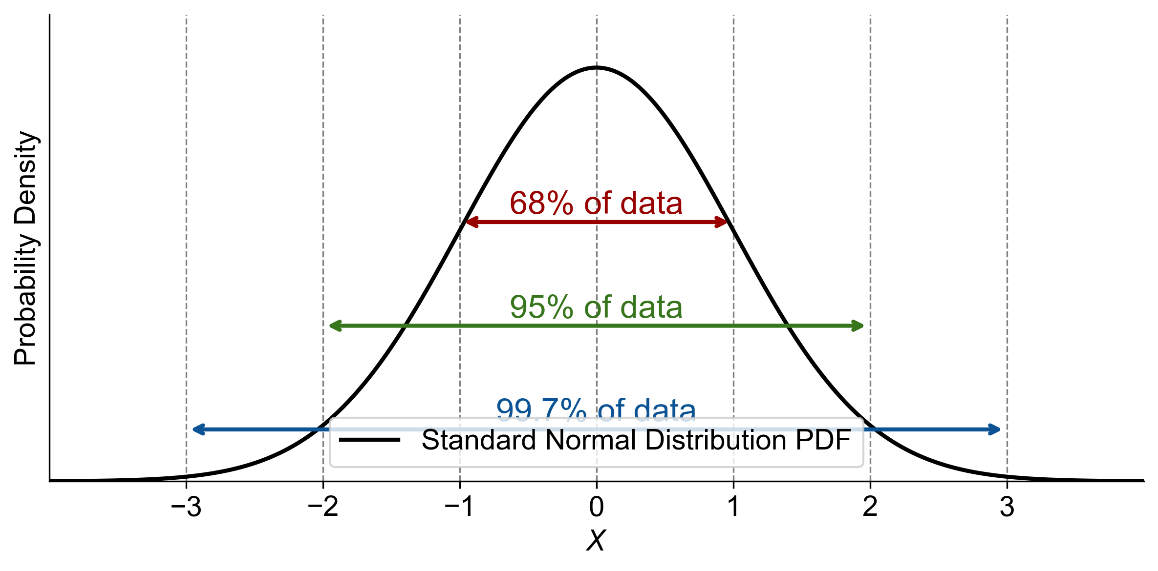
Fig. 5.21 Graphical representation of Standard Normal Distribution PDF highlighting key percentages of data within one, two, and three standard deviations from the mean.

5.4.3. Standardized Normally Distributed Variable

Understanding the transformation of normal distributions to standard normal distributions requires familiarity with z-scores. A z-score quantifies how many standard deviations an element is from the mean. The calculation of a z-score is given by:

(5.16)\[z = \dfrac{(X - \mu)}{\sigma}\]

Where:

• \(x\) represents a value from the original normal distribution.

• \(\mu\) denotes the mean of the original normal distribution.

• \(\sigma\) signifies the standard deviation of the original normal distribution.

The conversion process employs the z-score equation to standardize the data, resulting in a distribution with a mean (\(\mu\)) of 0 and a standard deviation (\(\sigma\)) of 1.

Recommended Steps

1. Identify the Original Distributions: Determine the mean (\(\mu\)) and standard deviation (\(\sigma\)) for each distribution.

2. Standardize Each Value: Utilize the z-score formula (5.16) to calculate the standardized value for each \(x\) in the original distributions.

By applying these steps, we can depict a standard normal distribution with \( \mu = 0 \) and \( \sigma = 1 \) on a graph.

Fig. 5.22 consists of three plots. The top plot shows five normal distributions with different means (\(\mu\)) and standard deviations (\(\sigma\)). The middle plot uses arrows to indicate the transformation of these distributions to the standard normal distribution, which is shown in the bottom plot.

Top Plot:

• Pink Curve: \(\mu\) = -2, \(\sigma\) = 1

• Green Curve: \(\mu\) = 0, \(\sigma\) = 0.5

• Blue Curve: \(\mu\) = 3, \(\sigma\) = 2

• Orange Curve: \(\mu\) = 6, \(\sigma\) = 1

• Purple Curve: \(\mu\) = 8, \(\sigma\) = 2/3

Middle Plot:

• Arrows indicate the transformation of each normal distribution to the standard normal distribution.

Bottom Plot:

• Green Curve: Standard normal distribution with \(\mu\) = 0 and \(\sigma\) = 1

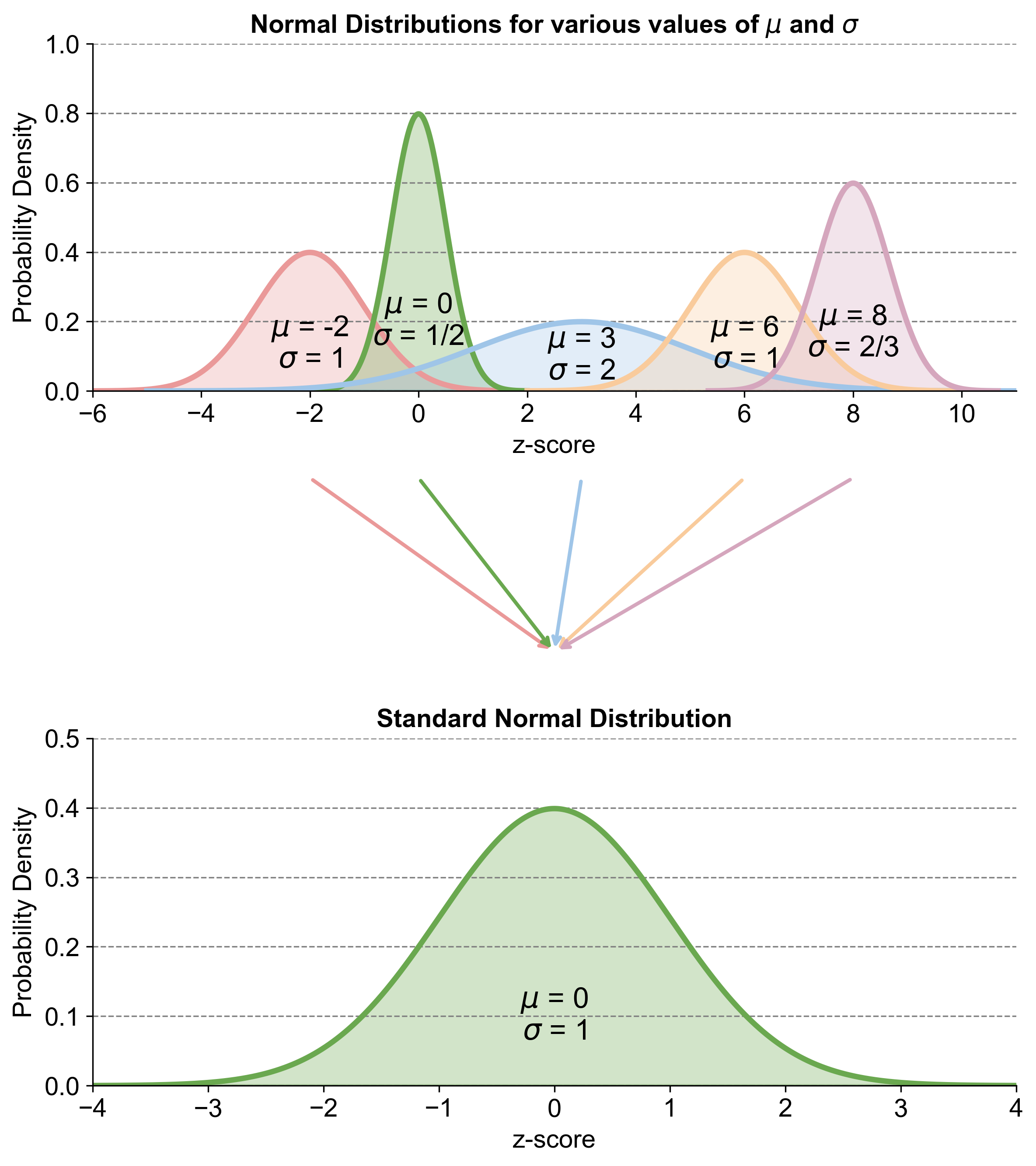
Fig. 5.22 Transformation of various normal distributions to a standard normal distribution using z-scores, highlighting the standardization process.

\(\mathbf{z}_{\mathbf{\alpha}}\) Notation

The symbol \(z_{\alpha}\) is used to denote the z-score that has an area of \(\alpha\) (alpha) to its right under the standard normal curve. Read “\(z_{\alpha}\)” as “z sub α” or more simply as “z \({\alpha}\)”.

5.4.4. Using a z-score Table

A z-score table displays the cumulative probability of a z-score in a standard normal distribution. The table is constructed under the assumption that the distribution has a mean (\(\mu\)) of 0 and a standard deviation (\(\sigma\)) of 1. The values in the table represent the area under the curve to the left of a given z-score.

Steps for Utilizing Our z-score Table

1. Identify the z-score: We begin by converting the raw score of interest into a z-score using the formula:

   \[\begin{equation*} z = \dfrac{(X - \mu)}{\sigma} \end{equation*}\]

   Here, \(x\) is the raw score, \(\mu\) is the mean of the distribution, and \(\sigma\) is the standard deviation.

2. Locate the z-score on Our Table: We find the row that aligns with the first two digits of the z-score and the column that matches the second decimal place. The intersection of this row and column reveals the cumulative probability.

3. Interpret the Table Value: The value we discover on the z-score table indicates the probability that a random variable falls below our z-score, representing the area to the left of the z-score on the curve.

4. Determine Greater Than Probabilities: To find the probability of a z-score exceeding a certain value, we subtract the table value from 1, considering the total area under the curve is 1.

5. Handle Negative z-scores: When dealing with negative z-scores, we utilize the symmetry of the standard normal distribution. The probability for a negative z-score equates to 1 minus the probability of the corresponding positive z-score.

5.4.4.1. Postive Side of z-score table

	0.0	0.01	0.02	0.03	0.04	0.05	0.06	0.07	0.08	0.09
z
Loading ITables v2.2.3 from the init_notebook_mode cell... (need help?)

5.4.4.2. Negative Side of z-score table

	0.09	0.08	0.07	0.06	0.05	0.04	0.03	0.02	0.01	0.0
z
Loading ITables v2.2.3 from the init_notebook_mode cell... (need help?)

Remark

The above z-distribution tables are also available in Section 8.1

Example 5.11

To determine \(P(Z < 2.05)\), which represents the probability of a z-score being less than 2.05, we use a z-score table. Here’s a step-by-step guide on how to use it effectively:

1. Identify the Target Z-score: Our goal is to find \(P(Z < 2.05)\), the probability for a z-score less than 2.05.

2. Decompose the Z-score: Split the z-score into its integer and decimal parts:

   • Integer part: 2.0

   • Decimal part: 0.05

3. Navigate the Z-score Table:

   • Find the row corresponding to the integer part (2.0).

   • Locate the column matching the decimal part (0.05).

4. Find the Cumulative Probability: The intersection of the identified row and column provides the cumulative probability. This value represents \(P(Z < 2.05)\), which is the area under the standard normal curve to the left of the z-score 2.05.

5. Visualize the Outcome: Imagine a standard normal curve:

   • The total area under the curve represents all possible outcomes (100%).

   • The shaded area to the left of \(z = 2.05\) represents \(P(Z < 2.05) = 0.9798\) or 97.98% of the data.

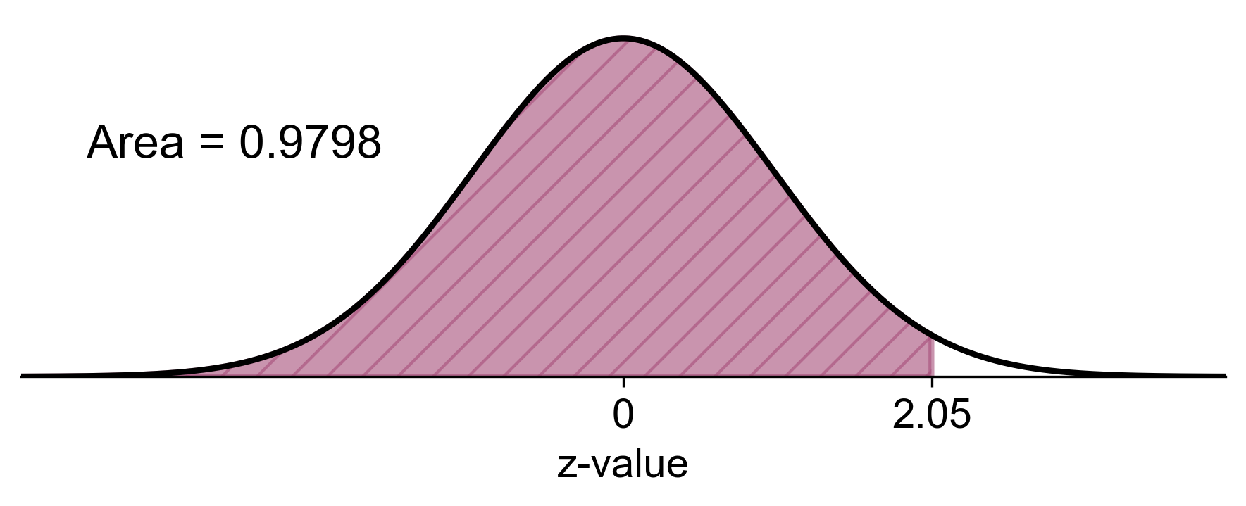
Fig. 5.23 Visual representation of \(P(Z < 2.05)\), showing the probability of a z-score being less than 2.05.

Note

For negative z-scores, the process remains the same due to the symmetry of the standard normal distribution. For instance, \(P(Z > -2.05)\) would be 1 - 0.9798 = 0.0202, representing the area to the left of -2.05 on the curve.

Three specific cases:

• (a) Area to the Left of a Specified z-score (Fig. 5.24 (a))

  • Process: To find the area to the left of a specified z-score \(z_1\), look up the z-score directly in the z-table.

  • Result: The table provides the cumulative probability \(P(Z \leq z_1)\) from the far left of the distribution up to the z-score, representing the area under the curve to the left of that score:

  \[\begin{equation*} \text{Area to the Left of } z_1 = P(Z \leq z_1). \end{equation*}\]

• (b) Area to the Right of a Specified z-score (Fig. 5.24 (b))

  • Process: To find the area to the right of a specified z-score \(z_1\), subtract the area to the left (found in the z-table) from 1.

  • Result: Since the total area under the curve is 1, this calculation gives the area to the right of the z-score:

  \[\begin{equation*} \text{Area to the Right of } z_1 = P(Z \geq z_1) = 1 - P(Z < z_1). \end{equation*}\]

• (c) Area Between Two Specified z-scores (Fig. 5.24 (c))

  • Process: To find the area between two specified z-scores \(z_1\) and \(z_2\) (where \(z_1 < z_2\)), subtract the area to the left of the lower z-score from the area to the left of the higher z-score.

  • Result: This difference gives the area under the curve between the two z-scores:

  \[\begin{equation*} \text{Area Between } z_1 \text{ and } z_2 = P(z_1 \leq Z \leq z_2) = P(Z \leq z_2) - P(Z < z_1). \end{equation*}\]

Fig. 5.24 Areas Under the Standard Normal Distribution Curve for (a) Area to the Left of a Specified z-score, (b) Area to the Right of a Specified z-score, and (c) Area Between Two Specified z-scores.

Example 5.12

If the random variable \(z\) has a standard normal distribution, sketch and find each of the following probabilities:

• a. \(P(0 \leq z \leq 1.5)\)

• b. \(P(z \geq 2)\)

• c. \(P(z \leq 1.5)\)

• d. \(P(z \geq -1)\)

Solution: To calculate the probabilities for the given conditions where \(z\) has a standard normal distribution, we can use the z-score table or a standard normal distribution calculator. Here are the probabilities:

a. \(P(0 \leq z \leq 1.5)\): This is the probability that \(z\) is between 0 and 1.5. We find the area to the left of \(z = 1.5\) and subtract the area to the left of \(z = 0\) (which is 0.5 since the total area under the curve is 1 and the curve is symmetrical around zero).

• Step 1: Find the area to the left of \(z = 1.5\) using the z-table.

• Step 2: Since \(z = 0\) is the mean of the standard normal distribution, the area to the left is 0.5.

• Step 3: Subtract the area to the left of \(z = 0\) from the area to the left of \(z = 1.5\).

• Calculation: \(P(z \leq 1.5) - P(z \leq 0) = 0.9332 - 0.5 = 0.4332\)

• Result: \(P(0 \leq z \leq 1.5) = 0.4332\)

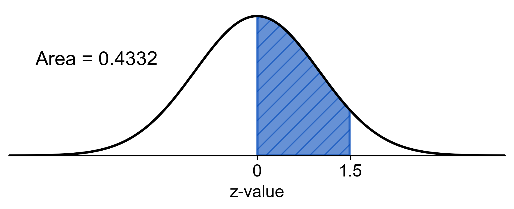
Fig. 5.25 Probability of \(z\) between 0 and 1.5 in a standard normal distribution

b. \(P(z \geq 2)\): This is the probability that \(z\) is greater than or equal to 2. We find the area to the left of \(z = 2\) and subtract it from 1 to get the area to the right.

• Step 1: Find the area to the left of \(z = 2\) using the z-table.

• Step 2: Subtract this value from 1 to get the area to the right.

• Calculation: \(P(z \geq 2) = 1 - P(z < 2) = 1 - 0.9772 = 0.0228\)

• Result: \(P(z \geq 2) = 0.0228\)

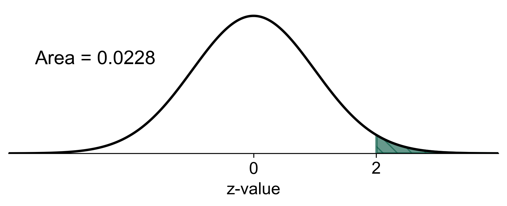
Fig. 5.26 Probability of \(z\) greater than or equal to 2 in a standard normal distribution

c. \(P(z \leq 1.5)\): This is the probability that \(z\) is less than or equal to 1.5. We find the area to the left of \(z = 1.5\).

• Step 1: Find the area to the left of \(z = 1.5\) using the z-table.

• Result: \(P(z \leq 1.5) = 0.9332\)

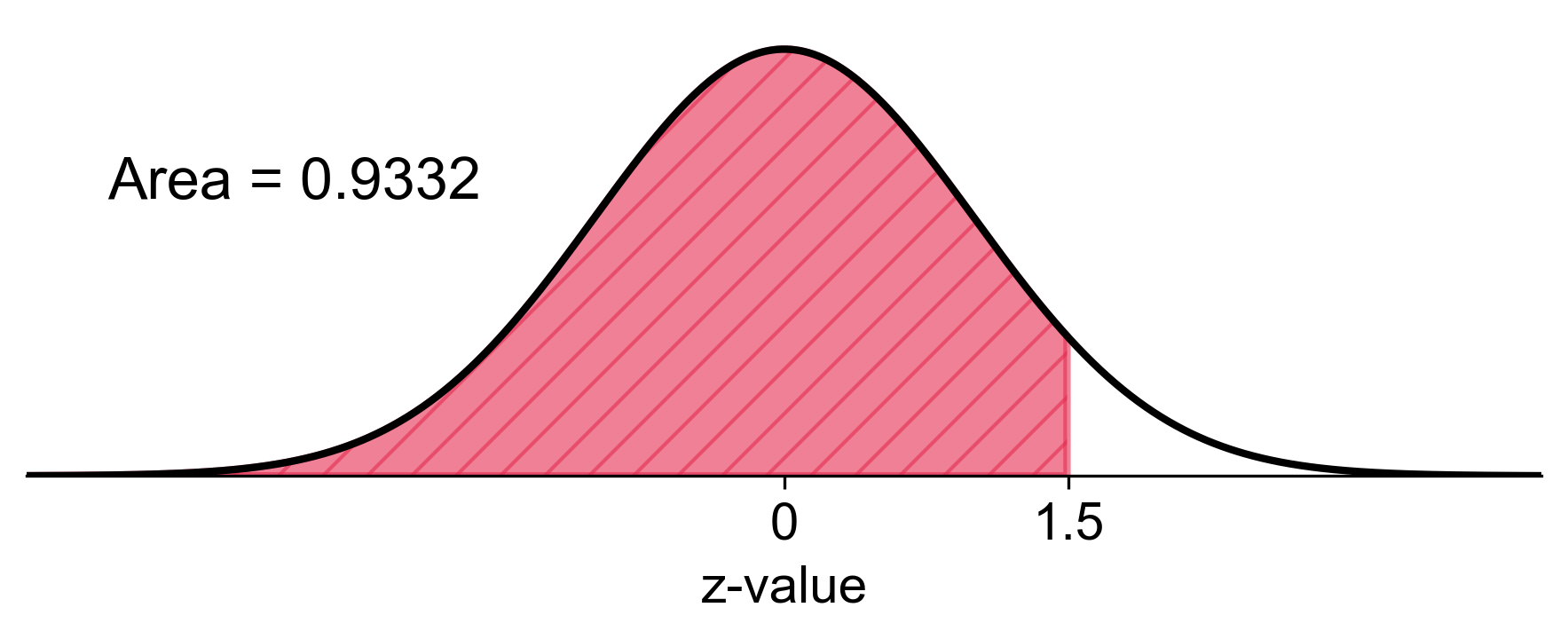
Fig. 5.27 Probability of \(z\) less than or equal to 1.5 in a standard normal distribution

d. \(P(z \geq -1)\): This is the probability that \(z\) is greater than or equal to -1. Since the curve is symmetrical, this is the same as the area to the left of \(z = 1\), which we can find directly from the table.

• Step 1: Find the area to the left of \(z = -1\) using the z-table.

• Step 2: Since the distribution is symmetrical, \(P(z \leq -1) = P(z \geq 1)\).

• Step 3: Subtract the area to the left of \(z = -1\) from 1.

• Calculation: \(P(z \geq -1) = 1 - P(z < -1) = 1 - 0.1587 = 0.8413\)

• Result: \(P(z \geq -1) = 0.8413\)

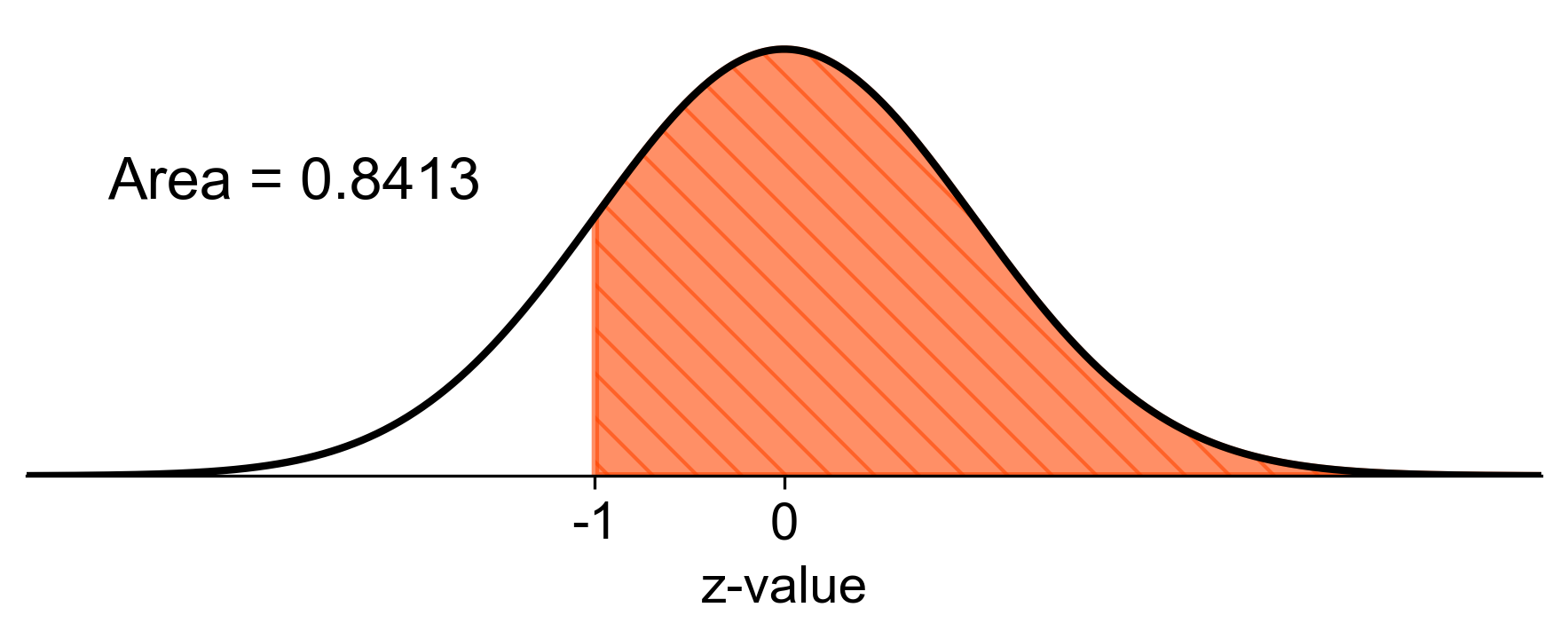
Fig. 5.28 Probability of \(z\) greater than or equal to -1 in a standard normal distribution

Example 5.13

If the random variable \(z\) has a standard normal distribution, find each of the following probabilities:

• a. \(P(-1.5 \leq z \leq 0)\)

• b. \(P(z \leq -2)\)

• c. \(P(-2 \leq z \leq 2)\)

• d. \(P(z > 1)\)

Solution:

a. \(P(-1.5 \leq z \leq 0)\)

• Step 1: Find the area to the left of \(z = -1.5\) using the z-table.

• Step 2: Since \(z = 0\) is the mean of the standard normal distribution, the area to the left is 0.5.

• Step 3: Subtract the area to the left of \(z = -1.5\) from the area to the left of \(z = 0\).

• Calculation: \(P(z \leq 0) - P(z < -1.5) = 0.5 - 0.0668 = 0.4332\)

• Result: \(P(-1.5 \leq z \leq 0) = 0.4332\)

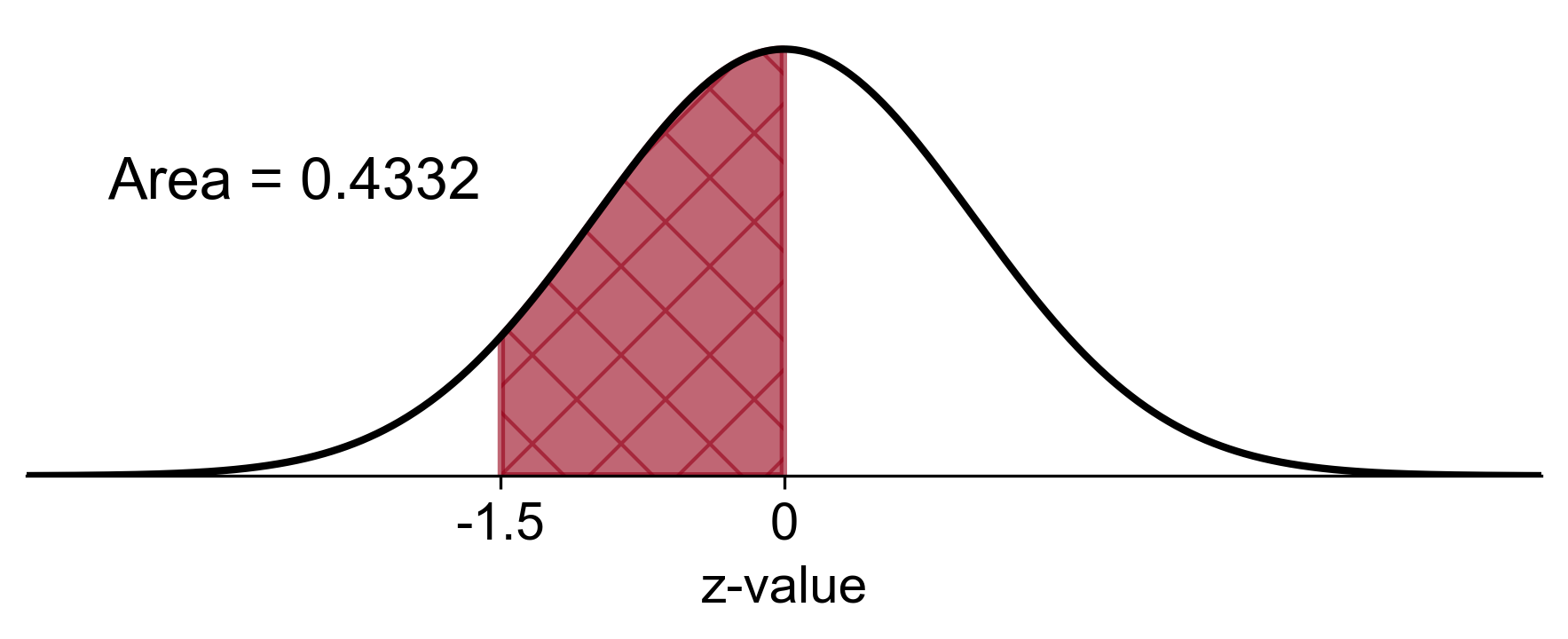
Fig. 5.29 Probability of \(z\) between -1.5 and 0 in a standard normal distribution

b. \(P(z \leq -2)\)

• Step 1: Find the area to the left of \(z = -2\) using the z-table.

• Result: \(P(z \leq -2) = 0.0228\)

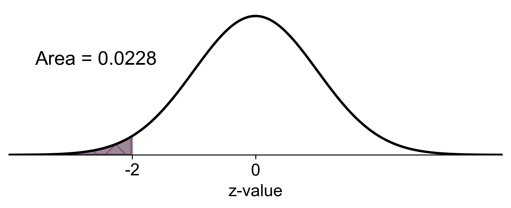
Fig. 5.30 Probability of \(z\) less than or equal to -2 in a standard normal distribution

c. \(P(-2 \leq z \leq 2)\)

• Step 1: Find the area to the left of \(z = 2\) using the z-table.

• Step 2: Find the area to the left of \(z = -2\) using the z-table.

• Step 3: Subtract the area to the left of \(z = -2\) from the area to the left of \(z = 2\).

• Calculation: \(P(z \leq 2) - P(z < -2) = 0.9772 - 0.0228 = 0.9544\)

• Result: \(P(-2 \leq z \leq 2) = 0.9544\)

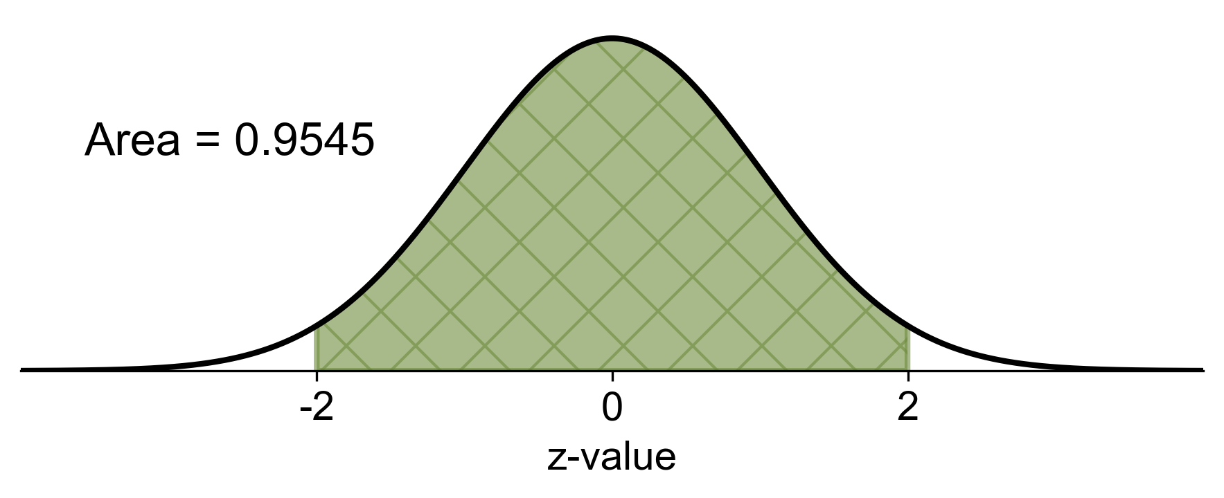
Fig. 5.31 Probability of \(z\) between -2 and 2 in a standard normal distribution

d. \(P(z > 1)\)

• Step 1: Find the area to the left of \(z = 1\) using the z-table.

• Step 2: Subtract this value from 1 to get the area to the right.

• Calculation: \(P(z > 1) = 1 - P(z \leq 1) = 1 - 0.8413 = 0.1587\)

• Result: \(P(z > 1) = 0.1587\)

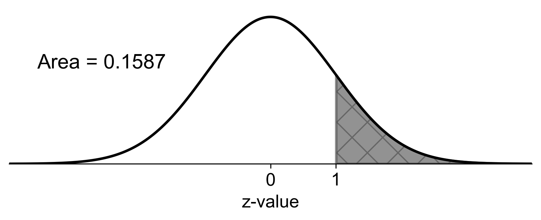
Fig. 5.32 Probability of \(z\) greater than 1 in a standard normal distribution

5.4.5. Interpreting z-scores for Tail Probabilities

In the context of statistics, z-scores are a fundamental concept, particularly within the standard normal distribution framework. They are instrumental in determining the relative position of data points by measuring how many standard deviations they are from the mean. This metric becomes crucial when assessing tail probabilities, which estimate the likelihood of observing values at the distribution’s extremes. The symbol \(z_{\alpha}\) is used to denote the z-score that has an area of α (alpha) to its right under the standard normal curve. Read “\(z_{\alpha}\)” as “z sub \(\alpha\)” or more simply as “z \(\alpha\).”

Tail probabilities are intimately linked with their corresponding z-scores. For instance, the right tail probability, denoted as \(P(Z > z)\), gauges the probability of a random variable exceeding a specific z-score. Conversely, the left tail area, \(P(Z \leq z)\), is simply one minus the right tail probability, reflecting the cumulative probability up to that z-score.

To illustrate, consider a right tail area of 0.025; the left tail area is then \(1 - 0.025 = 0.975\). The z-score associated with this left tail area can be located using a z-table or statistical software, often resulting in a value around 1.96.

Fig. 5.33 Illustration of z-score for a right tail area of 0.025 (left tail area of 0.975)

Similarly, a right tail area of 0.05 corresponds to a left tail area of \( 1 - 0.05 = 0.95 \), which typically aligns with a z-score near 1.645.

Fig. 5.34 Illustration of z-score for a right tail area of 0.05 (left tail area of 0.95)

These z-scores are not merely academic; they play a critical role in hypothesis testing. They represent critical values, or \( z_{\alpha} \), which are the thresholds for rejecting the null hypothesis. The subscript \( \alpha \), known as the significance level, is the probability of incorrectly rejecting a true null hypothesis.

Mathematically, finding \( z_{\alpha} \) involves solving the equation

(5.17)\[\begin{equation}P(Z > z_{\alpha}) = \alpha \end{equation}\]

where \( \alpha \) is the predetermined area in the distribution’s right tail. This calculation is essential for determining the z-score that serves as the cutoff for statistical significance in hypothesis testing. By solving this equation, we can ascertain the number of standard deviations a z-score must be from the mean to achieve a certain level of significance, thereby facilitating decision-making in statistical analyses.

Example 5.14

Complete the following table by finding the z-score that corresponds to each given right-tail area.

Right-Tail Area \(\alpha\)	Corresponding z-score
0.2	?
0.1	?
0.06	?
0.05	?
0.03	?
0.025	?
0.01	?
0.005	?

Solution:

a. Right-Tail Area of 0.2:

• Calculate the left-tail area: \( 1 - 0.2 = 0.8 \).

• Find the z-score that corresponds to a left-tail area of 0.8 in the z-table, which is approximately 0.84.

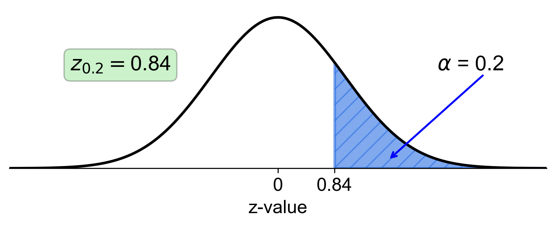
Fig. 5.35 Standard normal distribution with right-tail area of 0.2 and corresponding z-score of 0.84

b. Right-Tail Area of 0.1:

• Calculate the left-tail area: \( 1 - 0.1 = 0.9 \).

• Find the z-score that corresponds to a left-tail area of 0.9 in the z-table, which is approximately 1.28.

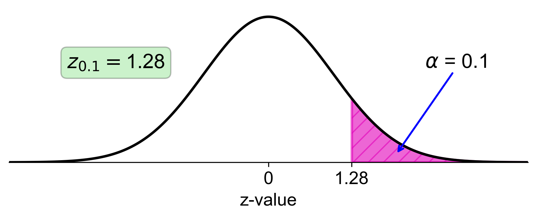
Fig. 5.36 Standard normal distribution with right-tail area of 0.1 and corresponding z-score of 1.28

c. Right-Tail Area of 0.06:

• Calculate the left-tail area: \( 1 - 0.06 = 0.94 \).

• Find the z-score that corresponds to a left-tail area of 0.94 in the z-table, which is approximately 1.555.

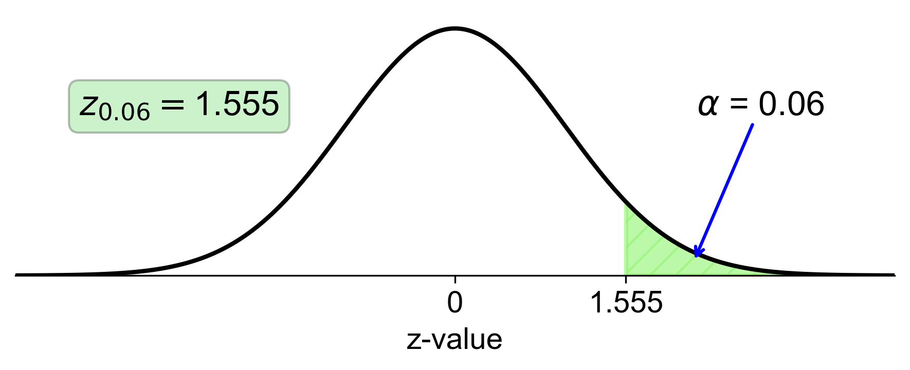
Fig. 5.37 Standard normal distribution with right-tail area of 0.06 and corresponding z-score of 1.555

d. Right-Tail Area of 0.05:

• Calculate the left-tail area: \( 1 - 0.05 = 0.95 \).

• Find the z-score that corresponds to a left-tail area of 0.95 in the z-table, which is approximately 1.64.

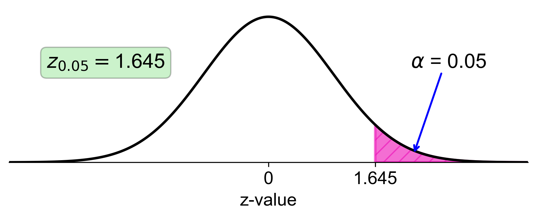
Fig. 5.38 Standard normal distribution with right-tail area of 0.05 and corresponding z-score of 1.64

e. Right-Tail Area of 0.03:

• Calculate the left-tail area: \( 1 - 0.03 = 0.97 \).

• Find the z-score that corresponds to a left-tail area of 0.97 in the z-table, which is approximately 1.88.

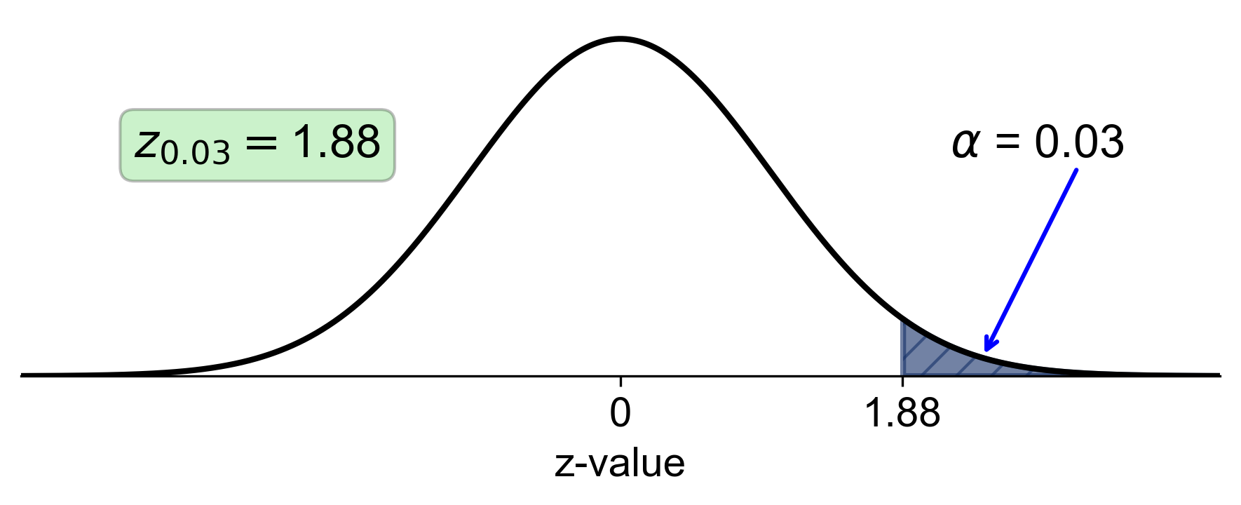
Fig. 5.39 Standard normal distribution with right-tail area of 0.03 and corresponding z-score of 1.88

f. Right-Tail Area of 0.025:

• Calculate the left-tail area: \( 1 - 0.025 = 0.975 \).

• Find the z-score that corresponds to a left-tail area of 0.975 in the z-table, which is approximately 1.96.

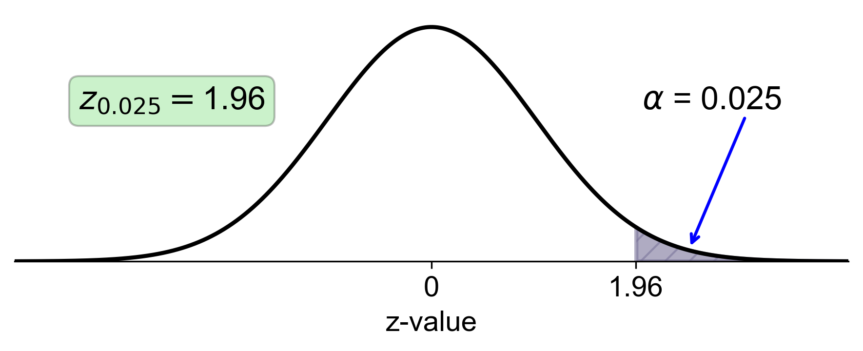
Fig. 5.40 Standard normal distribution with right-tail area of 0.025 and corresponding z-score of 1.96

g. Right-Tail Area of 0.01:

• Calculate the left-tail area: \( 1 - 0.01 = 0.99 \).

• Find the z-score that corresponds to a left-tail area of 0.99 in the z-table, which is approximately 2.33.

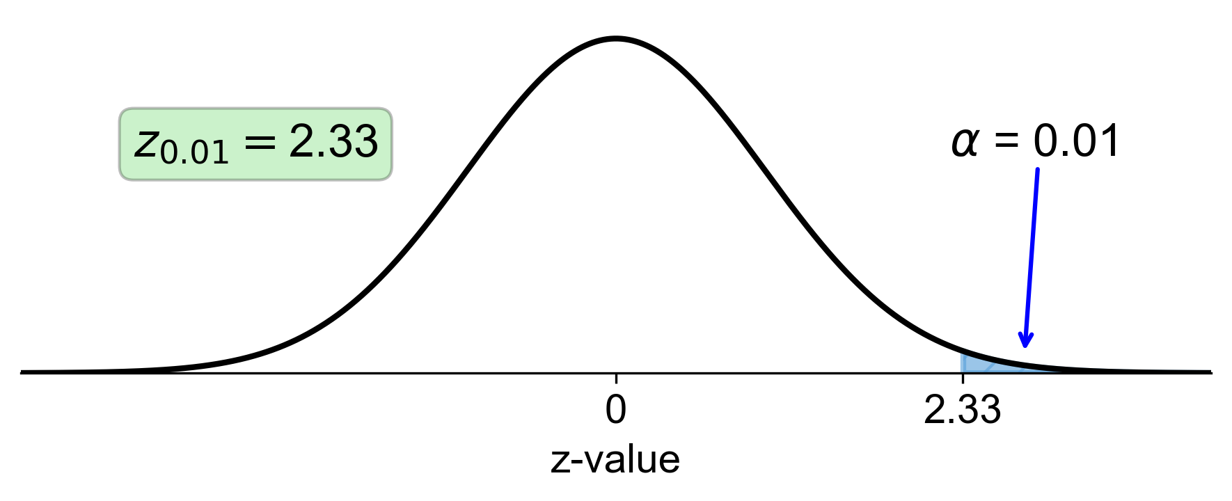
Fig. 5.41 Standard normal distribution with right-tail area of 0.01 and corresponding z-score of 2.33

h. Right-Tail Area of 0.005:

• Calculate the left-tail area: \( 1 - 0.005 = 0.995 \).

• Find the z-score that corresponds to a left-tail area of 0.995 in the z-table, which is approximately 2.58.

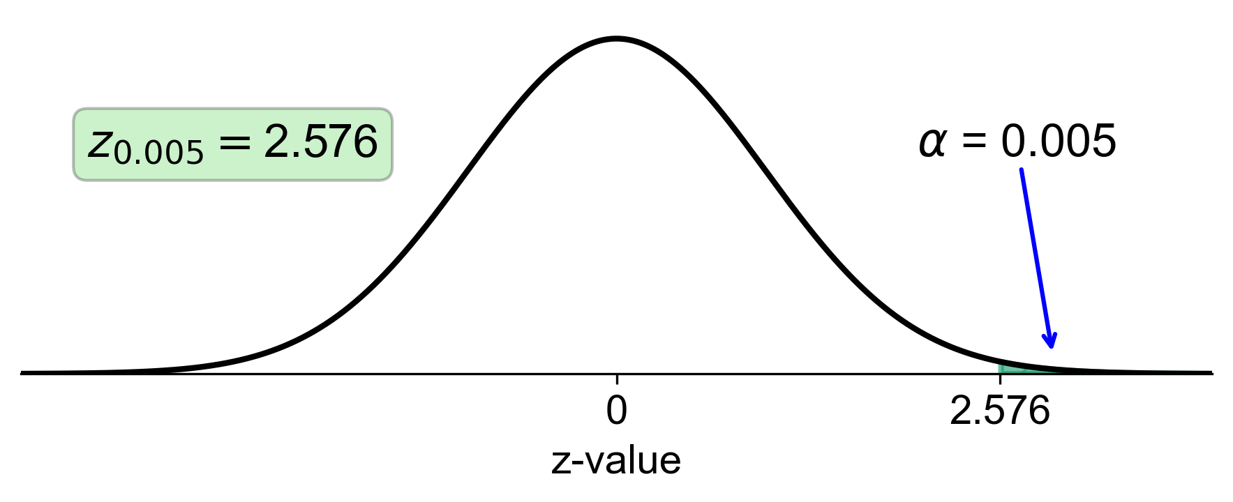
Fig. 5.42 Standard normal distribution with right-tail area of 0.005 and corresponding z-score of 2.58

Therefore,

Right-Tail Area	Corresponding z-score
0.2	0.84
0.1	1.28
0.06	1.555
0.05	1.645
0.03	1.88
0.025	1.96
0.01	2.33
0.005	2.576

5.4.6. Procedure for Calculating Probabilities in a Normal Distribution

To calculate the probability or percentage for a variable that follows a normal distribution, we can follow these steps:

1. Visualize the Distribution: Begin by drawing the normal curve that corresponds to the given variable. This curve represents the probability distribution of the variable.

2. Identify the Region of Interest: Shade the area under the curve that you’re interested in. This could be one or more regions, depending on the problem. Clearly mark the boundary value(s), known as the x-value(s), that delimit this region.

3. Convert to z-scores: Calculate the z-score(s) for the boundary x-value(s). The z-score is the number of standard deviations an x-value is from the mean of the distribution and is given by the formula:

   (5.18)\[\begin{equation} z = \dfrac{(X - \mu)}{\sigma} \end{equation}\]

   where \(x\) is the x-value, \(\mu\) is the mean, and \(\sigma\) is the standard deviation of the distribution.

4. Determine the Probability: Refer to the standard normal distribution table, often labeled as Table II, to find the probability associated with the z-score(s). This table provides the area under the curve to the left of a given z-score, which corresponds to the cumulative probability up to that point.

By following these steps, you can accurately determine the probability or percentage for any given range within a normal distribution.

Note

To translate a known z-score back to its corresponding x-value within a normal distribution, you can rearrange the standard z-score formula:

(5.19)\[\begin{equation} z = \dfrac{x - \mu}{\sigma} \end{equation}\]

Here, \(\mu\) represents the mean of the distribution, \(\sigma\) is the standard deviation, and \( z \) is the z-score. If you have the values for \(\mu\), \(\sigma\), and \( z \), you can solve for \(x\) using the following equation:

(5.20)\[\begin{equation} x = \mu + (z \cdot \sigma) \end{equation}\]

Keep in mind that if the z-score is to the left of the mean, it should be treated as a negative value in your calculations.

Example 5.15

Let \(\mu = 2\) and \(\sigma = 1.5\). If the random variable \(X\) has a standard normal distribution, determine the following probabilities:

• a. \(P(0 \leq X \leq 1.5)\)

• b. \(P(X \geq 2)\)

• c. \(P(X \leq 1.5)\)

• d. \(P(X \geq -1)\)

Solution:

• a. For part a, \(P(0 \leq X \leq 1.5)\):

  1. Convert to z-scores: We start by transforming the \(x\) values into z-scores using the formula: \begin{equation*} z = \dfrac{(X - \mu)}{\sigma} \end{equation*} This standardizes the \(x\) values, allowing us to use the standard normal distribution table.

  2. Calculate z-scores for Boundaries:

  • For \( X = 0 \), the z-score is:

    \[\begin{equation*} z = \dfrac{(0 - 2)}{1.5} = -1.33 \end{equation*}\]

  • For \( X = 1.5 \), the z-score is:

    \[\begin{equation*} z = \dfrac{(1.5 - 2)}{1.5} = -0.33 \end{equation*}\]

  3. Determine Probabilities:

  • The area to the left of \( z = -1.33 \) is approximately 0.0918.

  • The area to the left of \( z = -0.33 \) is approximately 0.3707.

  4. Find the Probability for the Range:

  • The probability that \(x\) is between 0 and 1.5 is the difference between the two areas:

    \[\begin{equation*} P(0 \leq X \leq 1.5) = 0.3707 - 0.0918 = 0.2789 \end{equation*}\]

  Therefore, the probability that the random variable \(x\) is between 0 and 1.5 is approximately 0.2789, or 27.89%. This calculation assumes that the values are looked up from a standard normal distribution table, which provides the cumulative probability up to a given z-score. The z-scores are negative because the values of \(x\) are less than the mean \(\mu\).

  

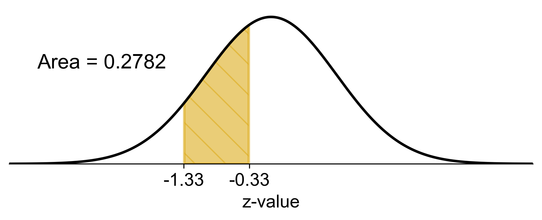
  Fig. 5.43 Visual representation of \(P(0 \leq X \leq 1.5)\) from Example 5.15 (a).

• b. For part b, we are interested in finding the probability that the random variable \(x\) is greater than or equal to 2, given that the mean \(\mu\) is also 2.

  Since \( X = 2 \) coincides with the mean of the distribution, and we know that a normal distribution is symmetric about its mean, exactly half of the distribution’s area lies to the right of the mean. Therefore, the probability that \(x\) is greater than or equal to 2 is simply the area to the right of the mean, which is 0.5.

  Thus, we can state that:

  \[\begin{equation*} P(X \geq 2) = 0.5 \end{equation*}\]

  This reflects the fundamental property of symmetry in a normal distribution, where the median, mean, and mode all coincide, dividing the distribution into two equal halves.

  

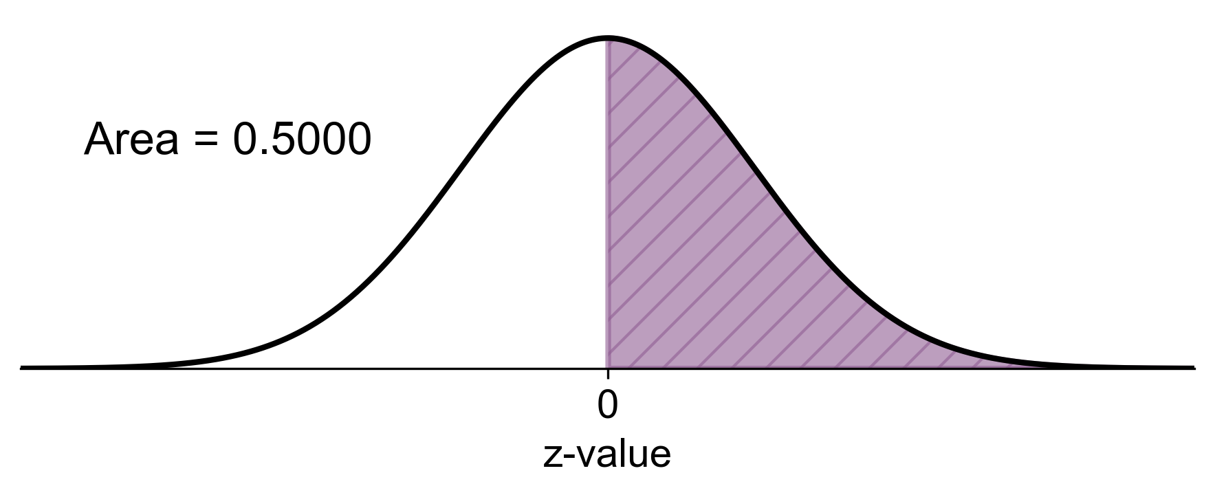
  Fig. 5.44 Visual representation of \(P(X \geq 2)\) from Example 5.15 (b).

• c. \( P(X \leq 1.5) \):

  1. Convert to z-score: Calculate the z-score for \( X = 1.5 \) using the formula:

  \[\begin{equation*} z = \dfrac{(X - \mu)}{\sigma} \end{equation*}\]

  where \(x\) is the raw score, \(\mu\) is the mean, and \(\sigma\) is the standard deviation.

  2. Calculate z-score: Substitute the values into the formula:

  \[\begin{equation*} z = \dfrac{(1.5 - 2)}{1.5} = -0.33 \end{equation*}\]

  3. Find Probability: Look up the z-score of -0.33 in the standard normal distribution table to find the cumulative probability to the left of this z-score.

  The area to the left of \( z = -0.33 \) is approximately 0.3707. Therefore, the probability that \(x\) is less than or equal to 1.5 is:

  \[\begin{equation*} P(X \leq 1.5) = 0.3707 \end{equation*}\]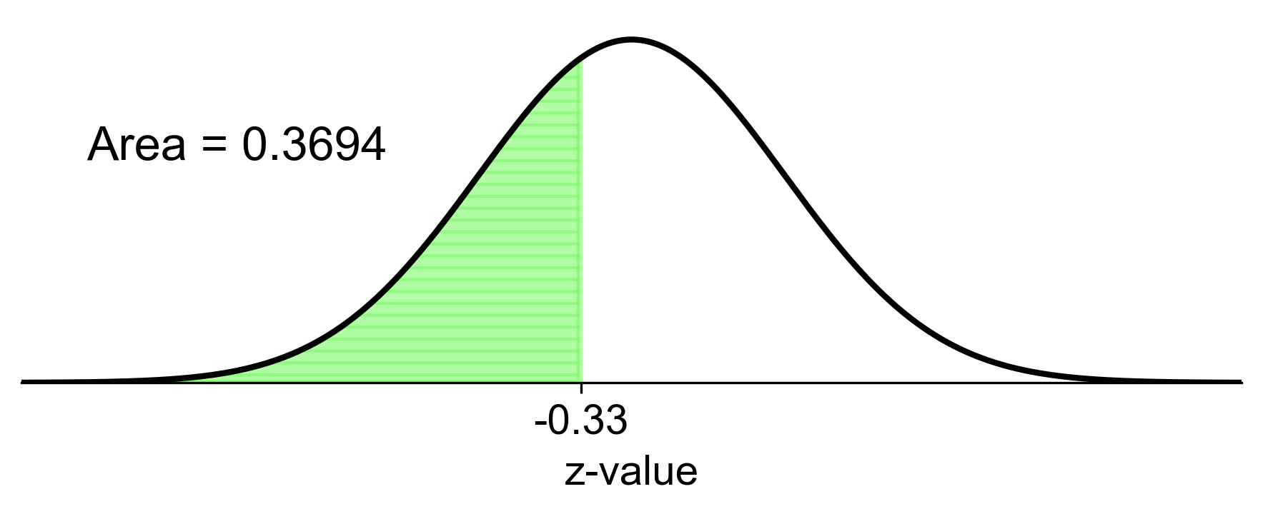

  

  Fig. 5.45 Visual representation of \(P(X \leq 1.5)\) from Example 5.15 (c).

• d. \( P(X \geq -1) \)

  1. Convert to z-score: Calculate the z-score for \( X = -1 \) using the formula:

  \[\begin{equation*} z = \dfrac{(X - \mu)}{\sigma} \end{equation*}\]

  where \(x\) is the raw score, \(\mu\) is the mean, and \(\sigma\) is the standard deviation.

  2. Calculate z-score: Substitute the values into the formula:

  \[\begin{equation*} z = \dfrac{(-1 - 2)}{1.5} = -2 \end{equation*}\]

  3. Find Probability: Look up the z-score of -2 in the standard normal distribution table to find the cumulative probability to the left of this z-score.

  The area to the left of \( z = -2 \) is approximately 0.0228. Therefore, the probability that \(x\) is greater than or equal to -1 is:

  \[\begin{equation*} P(X \geq -1) = 1 - 0.0228 = 0.9772 \end{equation*}\]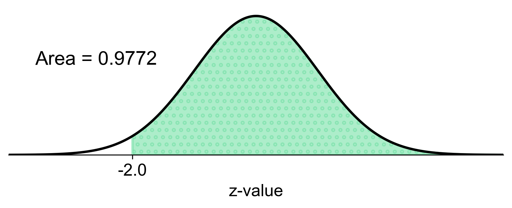

  

  Fig. 5.46 Visual representation of \(P(X \geq -1)\) from Example 5.15 (d).

Example 5.16

During a 20-day period, a population of daisy plants exhibited growth that was normally distributed with a mean (\(\mu\)) of 2.8 cm and a standard deviation (\(\sigma\)) of 0.45 cm. Determine the percentage of plants that grow:

• a. 3.5 cm or more?

• b. 2.8 cm or less?

• c. between 2.3 cm and 3.2 cm?

Solution: To find these percentages, we’ll use the z-score formula:

\[\begin{equation*} Z = \frac{X - \mu}{\sigma} \end{equation*}\]

where \(X\) is the value for which we’re finding the z-score, \(\mu\) is the mean, and \(\sigma\) is the standard deviation.

a) For plants growing 3.5 cm or more: \(P(X \geq 3.5)\)

\[\begin{equation*} Z = \frac{3.5 - 2.8}{0.45} = \frac{0.7}{0.45} \approx 1.56 \end{equation*}\]

Using the Z-table:

\[\begin{align*} P(X \geq 3.5) &= P(Z \geq 1.56) \\ &= 1 - P(Z < 1.56) \\ &= 1 - 0.9405 \\ &= 0.0595 \end{align*}\]

Therefore, approximately 5.95% of plants grow 3.5 cm or more.

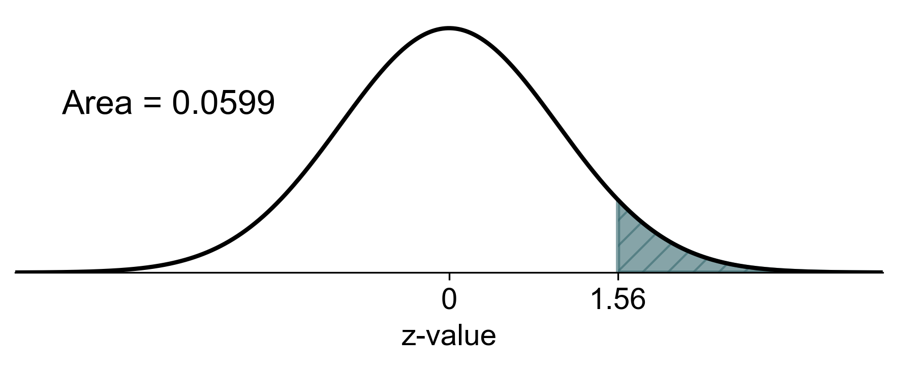
Fig. 5.47 Visual representation of the percentage of plants growing 3.5 cm or more (shaded area).

b) For plants growing 2.8 cm or less: \(P(X \leq 2.8)\) The z-score for 2.8 cm is 0 (because it’s the mean).

\[\begin{align*} P(X \leq 2.8) &= P(Z \leq 0) \\ &= 0.5 \end{align*}\]

Therefore, 50% of the plants grow 2.8 cm or less.

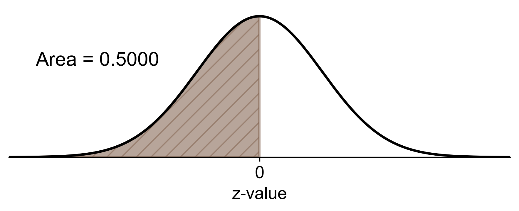
Fig. 5.48 Visual representation of the percentage of plants growing 2.8 cm or less (shaded area).

c) For plants growing between 2.3 cm and 3.2 cm: \(P(2.3 < X < 3.2)\) First, find the z-scores for both values.

For 2.3 cm:

\[\begin{equation*} Z_1 = \frac{2.3 - 2.8}{0.45} = \frac{-0.5}{0.45} \approx -1.11 \end{equation*}\]

For 3.2 cm:

\[\begin{equation*} Z_2 = \frac{3.2 - 2.8}{0.45} = \frac{0.4}{0.45} \approx 0.89 \end{equation*}\]

Using the Z-table:

\[\begin{align*} P(2.3 < X < 3.2) &= P(-1.11 < Z < 0.89) \\ &= P(Z < 0.89) - P(Z \leq -1.11) \\ &= 0.8136 - 0.1336 \\ &= 0.68 \end{align*}\]

Therefore, approximately 68% of the plants grow between 2.3 cm and 3.2 cm.

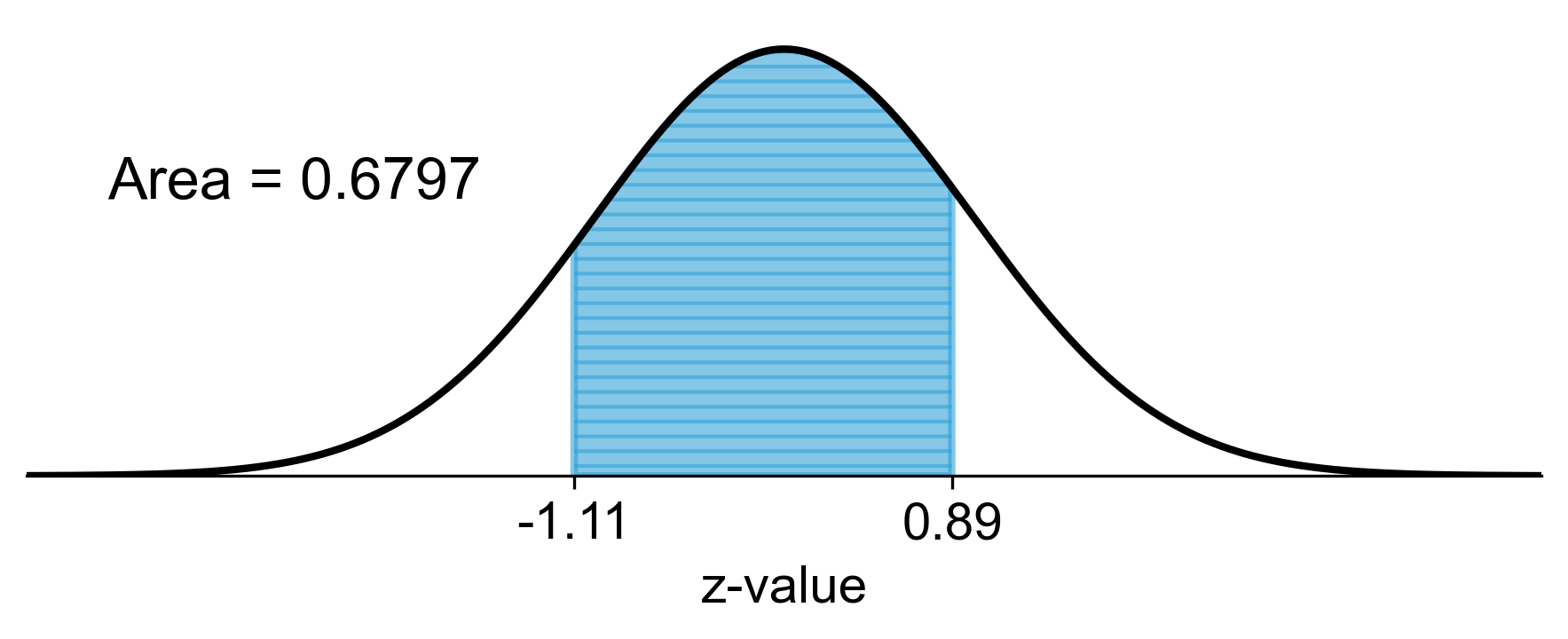
Fig. 5.49 Visual representation of the percentage of plants growing between 2.3 cm and 3.2 cm (shaded area).

Calculating Percentile from a Z-Score

To determine the percentile corresponding to a z-score in a standard normal distribution:

1. Find the Cumulative Probability: Use a z-table or statistical software to find the cumulative probability for the given z-score, regardless of whether it’s positive or negative. This represents the proportion of data points lying below the given z-score.

2. Convert to Percentile: Multiply the cumulative probability by 100 to express it as a percentile.

Example 5.17

Calculate the percentile for a student’s test score that has a z-score of -1.25.

Solution:

1. Cumulative Probability: To determine the percentile, we need to find \(P(Z \leq -1.25)\). Using the standard normal distribution table:

   For \(z = -1.25\), we find the cumulative probability directly from the table.

   \[P(Z \leq -1.25) \approx 0.1056\]

2. Percentile Conversion: The cumulative probability is already the percentile in decimal form. We convert this to a percentage:

   \[\text{Percentile} = 0.1056 \times 100 \approx 10.56\%\]

Therefore, the percentile rank for a z-score of -1.25 is approximately 10.56%. This means that approximately 10.56% of scores are at or below this value.

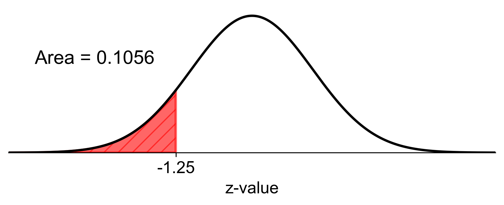
Fig. 5.50 Visual representation of the percentile for a z-score of -1.25 (shaded area).

If we need to present the percentile as a whole number, it would be rounded to 11%.

Example 5.18

Final exam scores in a mathematics course are normally distributed with a mean of 66 and a standard deviation of 7. Based on the above information and a Z-table, fill in the blanks in the table below.

Exam score	Z-score	Percentile
50
	-1.2
		90%

Solution: To complete the table, we’ll use the given information and the z-score formula.

Exam score	Z-score	Percentile
50	-2.29	1.11%
57.60	-1.2	11.51%
74.97	1.28	90%

Calculations:

1. For the Exam Score of 50:

   • Z-score: \(Z = \frac{X - \mu}{\sigma} = \frac{50 - 66}{7} \approx -2.29\)

   • Percentile: 1.11%

2. For the Z-score of -1.2:

   • Exam Score: \(X = Z \cdot \sigma + \mu = -1.2 \cdot 7 + 66 = 57.60\)

   • Percentile: 11.51%

3. For the Percentile of 90% (0.9):

   • Z-score: 1.28

   • Exam Score: \(X = Z \cdot \sigma + \mu = 1.28 \cdot 7 + 66 = 74.97\)

Explanations:

1. An exam score of 50 is 2.29 standard deviations below the mean, placing it at the 1.11th percentile.

2. A z-score of -1.2 corresponds to an exam score of 57.60, which is at the 11.51st percentile.

3. The 90th percentile (0.9) corresponds to a z-score of 1.28, which translates to an exam score of 74.97.

Example 5.19

BlueSky Air boasts a commendable on-time arrival rate, with 90% of its flights arriving as scheduled. To evaluate this claim, a sample of 16 BlueSky Air flights is randomly selected to observe their punctuality.

• a. Determine the exact probability that exactly 2 out of the 16 selected flights arrive late. Carry all intermediate calculations to at least six decimal places and provide the final answer rounded to three decimal places.

• b. Calculating the exact probability that 8 or more flights arrive late can be complex. Instead, we’ll employ the Normal approximation to estimate this probability. Ensure all intermediate values are calculated to at least six decimal places, and round the final answer to three decimal places.

Solution:

a.

The probability of exactly 2 flights arriving late is calculated using the binomial distribution formula:

\[\begin{equation*} P(X = x) = \binom{n}{x} p^x (1 - p)^{n - x} \end{equation*}\]

For \( n = 16 \) flights, \( x = 2 \) late arrivals, and the probability of a late arrival \( p = 0.1 \) (since \( p = 1 - 0.9 \)), we have:

\[\begin{equation*} P(X = 2) = \binom{16}{2} (0.1)^2 (0.9)^{14} \end{equation*}\]

\[\begin{equation*} P(X = 2) = \dfrac{16!}{2!(16 - 2)!} (0.1)^2 (0.9)^{14} \end{equation*}\]

\[\begin{equation*} P(X = 2) = 120 \times 0.01 \times 0.22876792454961 \end{equation*}\]

\[\begin{equation*} P(X = 2) = 0.274877906944 \end{equation*}\]

Thus, the exact probability that 2 flights arrive late is 0.275 (rounded to three decimal places).

b.

For the Normal approximation, we calculate the mean \(\mu\) and standard deviation \(\sigma\) for the binomial distribution:

\[\begin{equation*} \mu = np \end{equation*}\]

\[\begin{equation*} \sigma = \sqrt{np(1 - p)} \end{equation*}\]

With \( \mu = 16 \times 0.1 = 1.6 \) and \( \sigma = \sqrt{16 \times 0.1 \times 0.9} = 1.2 \).

To approximate the probability of at least 8 late flights, we apply a continuity correction and standardize the value:

\[\begin{equation*}z = \dfrac{x - \mu}{\sigma}= \dfrac{8 - 1.6}{1.2}= 5.33\end{equation*}\]

Using the standard normal distribution, we find:

\[\begin{equation*} P(X \geq 8) = P\left(Z \geq \dfrac{8 - 1.6}{1.2}\right) = P(Z \geq 5.33) \end{equation*}\]

Given the high z-score, the probability is exceedingly small and effectively 0 when rounded to three decimal places.

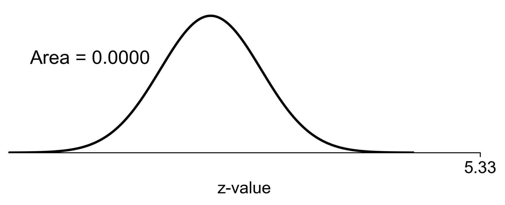
Fig. 5.51 Visual representation of the probability that 8 or more flights arrive late (shaded area).

Therefore, the approximated probability that at least 8 flights arrive late is 0.000 (rounded to three decimal places).

Example 5.20

TechGadget Inc. claims that 80% of their new gadgets pass the quality control tests. To verify this claim, a sample of 25 gadgets is randomly selected to observe their quality.

• a. Determine the exact probability that exactly 4 out of the 25 selected gadgets fail the quality control tests. Carry all intermediate calculations to at least six decimal places and provide the final answer rounded to three decimal places.

• b. Calculate the approximate probability that 7 or more gadgets fail the quality control tests using the Normal approximation. Ensure all intermediate values are calculated to at least six decimal places, and round the final answer to three decimal places.

Solution:

a.

The probability of exactly 4 gadgets failing the quality control tests is calculated using the binomial distribution formula:

\[\begin{equation*}P(X = x) = \binom{n}{x} p^x (1 - p)^{n - x}\end{equation*}\]

For \(n = 25\) gadgets, \(x = 4\) failures, and the probability of a failure \(p = 0.2\) (since \(p = 1 - 0.8\)), we have:

\[\begin{equation*}P(X = 4) = \binom{25}{4} (0.2)^4 (0.8)^{21}\end{equation*}\]

\[\begin{equation*}P(X = 4) = \dfrac{25!}{4!(25 - 4)!} (0.2)^4 (0.8)^{21}\end{equation*}\]

\[\begin{equation*}P(X = 4) = 12650 \times 0.0016 \times 0.0092233720\end{equation*}\]

\[\begin{equation*}P(X = 4) = 0.186681\end{equation*}\]

Thus, the exact probability that 4 gadgets fail the quality control tests is 0.233 (rounded to three decimal places).

b.

For the Normal approximation, we calculate the mean \(\mu\) and standard deviation \(\sigma\) for the binomial distribution:

\[\begin{equation*}\mu = np\end{equation*}\]

\[\begin{equation*}\sigma = \sqrt{np(1 - p)}\end{equation*}\]

With \(\mu = 25 \times 0.2 = 5\) and \(\sigma = \sqrt{25 \times 0.2 \times 0.8} = 2\).

To approximate the probability of at least 7 failures, we apply a continuity correction and standardize the value:

\[\begin{equation*}z = \dfrac{7 - \mu}{\sigma} = \dfrac{7 - 5}{2} = 1\end{equation*}\]

Using the standard normal distribution, we find:

\[\begin{equation*}P(X \geq 7) = P\left(Z \geq \dfrac{7 - 5}{2}\right) = P(Z \geq 1)\end{equation*}\]

Using the standard normal table or a calculator, we find:

\[\begin{equation*}P(Z \geq 1) = 1 - P(Z < 1) = 1 - 0.8413 = 0.1587\end{equation*}\]

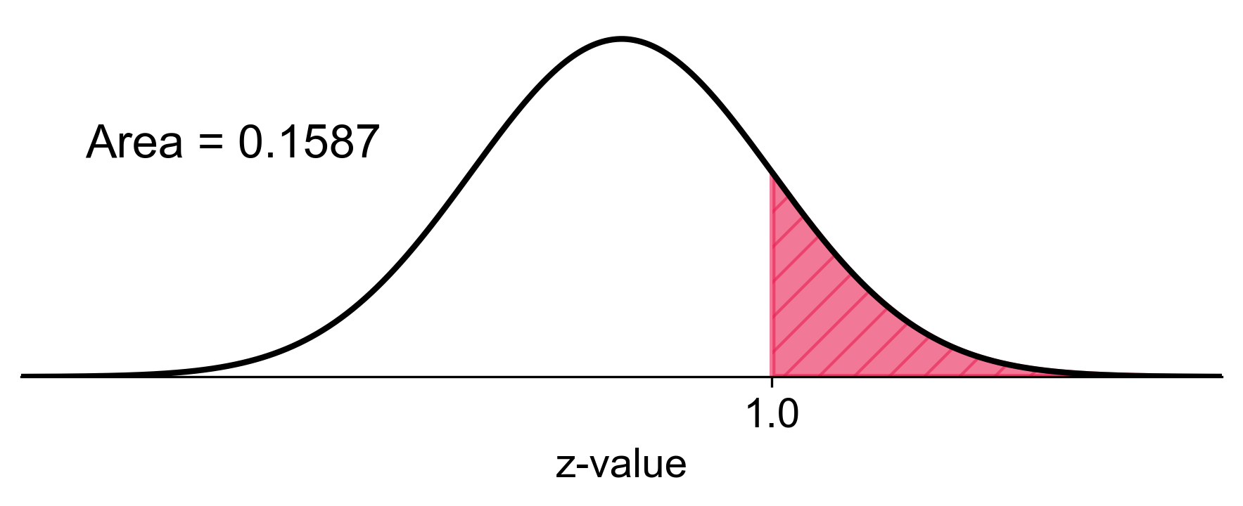
Fig. 5.52 Visual representation of the probability that 7 or more gadgets fail the quality control tests (shaded area).

Therefore, the approximated probability that at least 7 gadgets fail the quality control tests is 0.159 (rounded to three decimal places).