4.1. Probability Distribution Function (PDF) for a Discrete Random Variable#
4.1.1. Random Variable#
A random variable is a fundamental concept in probability and statistics. It essentially serves as a function that assigns a numerical value to each possible outcome of a random experiment [Shankar, 2021].
When you perform an experiment, like flipping a coin or rolling a die, there are multiple possible outcomes. A random variable provides a way to quantify these outcomes. For instance, if you flip a coin, you can define a random variable \(X\) such that \(X = 0\) if the outcome is tails and \(X = 1\) if the outcome is heads.
Definition - Random Variable
A random variable is a function that assigns a numerical value to each outcome of a random experiment. It maps outcomes from the sample space (the set of all possible results) to real numbers, allowing us to perform mathematical analysis and probability calculations.
Types of Random Variables:
There are two main types of random variables:
Discrete Random Variable: This type of random variable has a finite or countably infinite set of values it can assume. These values are distinct and separate, often representing countable outcomes.
Examples:
Number of heads in 10 coin tosses: Possible values are 0, 1, 2, …, 10.
Daily customer count at a cafe: Values could be 0, 1, 2, …, n, where n is the maximum capacity of the cafe.
Continuous Random Variable: A continuous random variable can take on any value within a given range or interval. The possibilities are infinite and uncountable, typically associated with measurements.
Examples:
Height of adults in a city: Any value within a realistic range, say from 140 cm to 200 cm.
Amount of water in a jug: Any value from 0 liters up to the jug’s capacity, measured precisely.
Understanding Random Variables:
The value of a random variable is realized only after the random experiment is conducted. For example, before we flip a coin, we don’t know if we’ll get a head or a tail—each outcome is determined by chance.
Discrete Example: Consider a lottery where the random variable \(X\) represents the number of matching numbers on a ticket. \(X\) can take on values 0, 1, 2, 3, 4, 5, or 6, each corresponding to the number of matches.
Continuous Example: If we measure the time \(T\) it takes for a chemical reaction to complete, \(T\) is a continuous random variable because it can take any value within a range, say from 0 to 10 minutes, depending on various factors like temperature and concentration.
4.1.2. Probability Mass Function (PMF) for a Discrete Random Variable#
The Probability Mass Function (PMF) is a function that gives the probability of a discrete random variable taking on a specific value. In other words, it maps each value of the random variable to its corresponding probability of occurrence. For a discrete random variable \(X\), the PMF is typically denoted as \(P(X = x)\) or \(p_X(x)\), where \(x\) represents a specific value that \(X\) can take [Devore et al., 2021].
Definition - Probability Mass Function (PMF)
The Probability Mass Function (PMF) of a discrete random variable \(X\) is a function that gives the probability that \(X\) will take on a particular value \(x\). It is typically denoted as \(P(X = x)\) or \(p_X(x)\), and is defined as:
where \(\text{Pr}(X = x)\) represents the probability that the random variable \(X\) equals \(x\).
Example 4.1 (Example of PMF - Coin Toss)
For coin flips, let \(X\) be the number of heads in one coin flip:
\(X\) (Number of Heads) |
\(P(X)\) (Probability) |
|---|---|
0 |
1/2 |
1 |
1/2 |
The Probability Mass Function (PMF) here tells us:
\(P(X = 0) = 1/2\) (probability of getting 0 heads)
\(P(X = 1) = 1/2\) (probability of getting 1 head)
This PMF completely describes the probability distribution for the random variable X, which represents the number of heads in a single fair coin flip.
Interpretation
There’s a 50% chance of getting no heads (i.e., getting a tail).
There’s a 50% chance of getting one head.
The probabilities sum to 1, as required for a valid PMF.
The PMF satisfies the following conditions:
Non-Negativity: The probability mass function values are non-negative for all possible values of X:
Summation: The sum of the probabilities over all possible values of X is equal to 1:
Where \(\mathcal{X}\) denotes the set of all possible values that the random variable X can take.
The PMF can be represented in various ways:
Table: A list of possible values of X and their corresponding probabilities.
Histogram: A graphical representation where each bar’s height represents the probability of a specific value.
Formula: A mathematical expression that gives the probability for any value of X.
Definitions - Probability Histogram
A probability histogram is a graphical representation of the probability distribution for a discrete random variable. It displays the possible values of the random variable on the horizontal axis and the probabilities associated with each value on the vertical axis. Each value is represented by a vertical bar whose height corresponds to the probability of that value occurring. The bars are typically disjoint and are spaced according to the gaps between the values of the discrete random variable.
Probability histograms are a visual tool used to understand and analyze the probabilities of different outcomes in a discrete random variable. They allow us to observe the relative likelihood of each value occurring and identify the most probable outcomes. Probability histograms can be useful for decision-making, risk assessment, and understanding the behavior of random processes.
To construct the probability histogram, we follow these steps:
Identify the possible values of X: Determine all the distinct values that the “number of siblings” variable X can take based on the data collected from the students.
Calculate the probabilities: Use the \(f/N\) rule, as mentioned before, to compute the probabilities for each value of X. Divide the frequency (\(f\)) of each value by the total number of observations (\(N\)) to obtain the probability of that specific value.
Plotting the histogram: On the horizontal axis, mark the possible values of X (e.g., 0, 1, 2, 3, etc.). On the vertical axis, represent the probabilities corresponding to each value as vertical bars. The height of each bar will be proportional to the probability of the respective value.
Ensuring appropriate scaling: To ensure that the histogram accurately represents the probabilities, make sure that the vertical axis is appropriately scaled to accommodate the probabilities ranging from 0 to 1.
Example 4.2 (Probability Mass Function and Histogram of a Fair Coin Flip)
When you flip a fair coin, the random variable “X” can take on only two values: 0 (for tails) and 1 (for heads). The probability mass function (PMF) for this discrete random variable is given by:
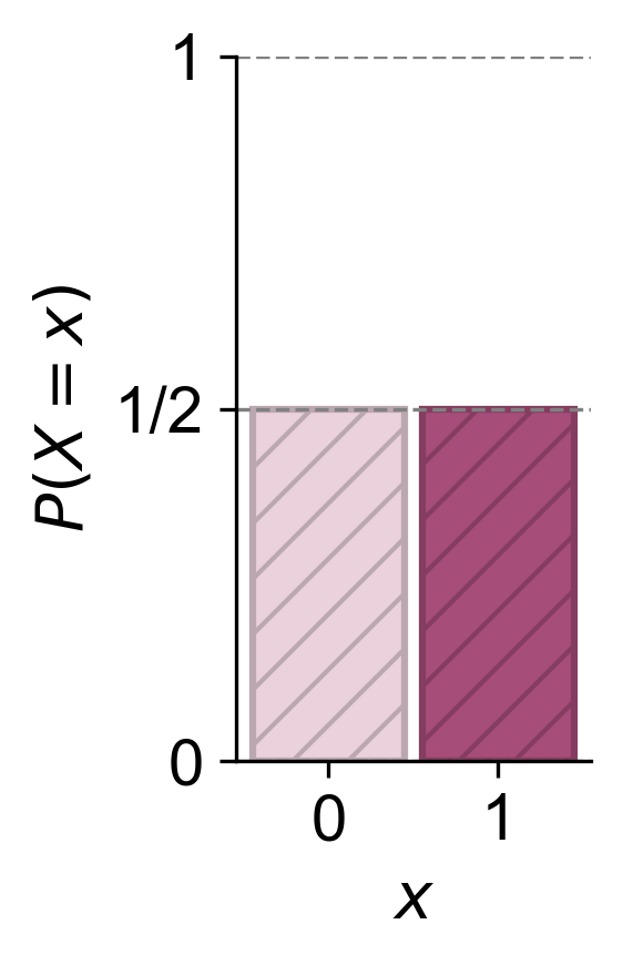
Fig. 4.1 The probability mass function (PMF) for a fair coin flip. The random variable “X” can take on two values: 0 (for tails) and 1 (for heads). Each outcome has an equal probability of 0.5, as shown by the bars reaching a height of 0.5 on the y-axis.#
Example 4.3 (Probability Mass Function and Histogram of a Fair Six-Sided Die Roll)
When you roll a standard six-sided die, the random variable “Y” can take on values from 1 to 6. The PMF for this discrete random variable is uniform because each outcome is equally likely:
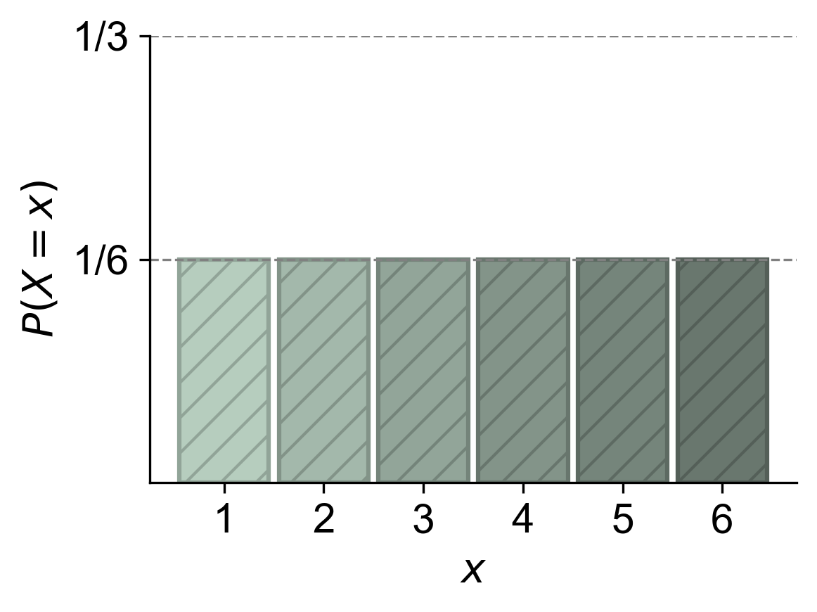
Fig. 4.2 The probability mass function (PMF) for rolling a standard six-sided die. The random variable “Y” can take on values from 1 to 6, with each outcome being equally likely. The height of each bar is \(\dfrac{1}{6}\), indicating that the probability of rolling any specific number (1 through 6) is the same, \(\dfrac{1}{6}\).#
Example 4.4 (PMF and Probability Histogram of Defective Items in a Batch)
Let’s say we are inspecting a batch of products, and the random variable “Z” represents the number of defective items in the batch. The values Z can take are non-negative integers (0, 1, 2, 3, …). The PMF might look like this:
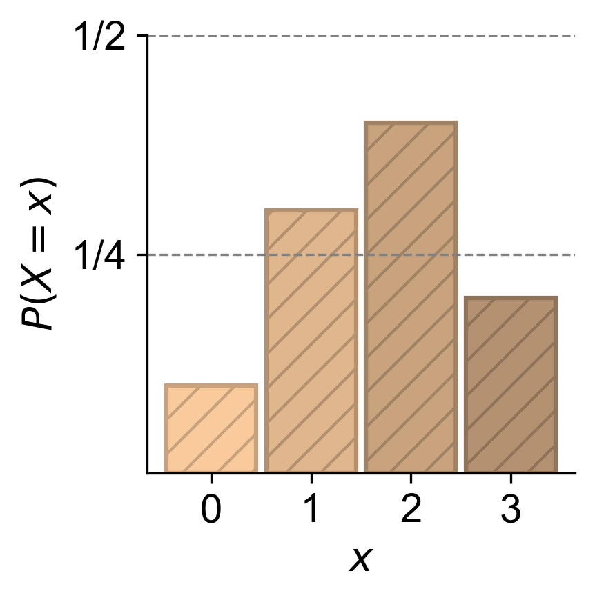
Fig. 4.3 The probability mass function (PMF) for the number of defective items, \(Z\), in a batch of products. The random variable \(Z\) can take on values 0, 1, 2, and 3, with the corresponding probabilities: \(P(Z = 0) = 0.1\) (10% chance of no defective items), \(P(Z = 1) = 0.3\) (30% chance of one defective item), \(P(Z = 2) = 0.4\) (40% chance of two defective items), and \(P(Z = 3) = 0.2\) (20% chance of three defective items).#
Example 4.5 (PMF and Probability Histogram for Drawing Balls Without Replacement)
Suppose you have a bag with 10 balls: 7 red balls and 3 blue balls. You randomly pick balls without replacement until you get a blue one. The random variable “W” represents the number of red balls picked. The values W can take are non-negative integers (0, 1, 2, 3, …, 7). The PMF can be calculated based on the probabilities of different scenarios.
Let’s calculate the PMF for W:
P(W = 0): The probability of picking a blue ball on the first draw.
\[\begin{equation*} P(W = 0) = \dfrac{3}{10} \end{equation*}\]P(W = 1): The probability of picking one red ball first, then a blue ball.
\[\begin{equation*} P(W = 1) = \dfrac{7}{10} \times \dfrac{3}{9} = \dfrac{7}{30} \end{equation*}\]P(W = 2): The probability of picking two red balls first, then a blue ball.
\[\begin{equation*} P(W = 2) = \dfrac{7}{10} \times \dfrac{6}{9} \times \dfrac{3}{8} = \dfrac{7}{40} \end{equation*}\]P(W = 3): The probability of picking three red balls first, then a blue ball.
\[\begin{equation*} P(W = 3) = \dfrac{7}{10} \times \dfrac{6}{9} \times \dfrac{5}{8} \times \dfrac{3}{7} = \dfrac{1}{8} \end{equation*}\]P(W = 4): The probability of picking four red balls first, then a blue ball.
\[\begin{equation*} P(W = 4) = \dfrac{7}{10} \times \dfrac{6}{9} \times \dfrac{5}{8} \times \dfrac{4}{7} \times \dfrac{3}{6} = \dfrac{1}{12} \end{equation*}\]P(W = 5): The probability of picking five red balls first, then a blue ball.
\[\begin{equation*} P(W = 5) = \dfrac{7}{10} \times \dfrac{6}{9} \times \dfrac{5}{8} \times \dfrac{4}{7} \times \dfrac{3}{6} \times \dfrac{2}{5} = \dfrac{1}{20} \end{equation*}\]P(W = 6): The probability of picking six red balls first, then a blue ball.
\[\begin{equation*} P(W = 6) = \dfrac{7}{10} \times \dfrac{6}{9} \times \dfrac{5}{8} \times \dfrac{4}{7} \times \dfrac{3}{6} \times \dfrac{2}{5} \times \dfrac{1}{4} = \dfrac{1}{40} \end{equation*}\]P(W = 7): The probability of picking all seven red balls first, then a blue ball.
\[\begin{equation*} P(W = 7) = \dfrac{7}{10} \times \dfrac{6}{9} \times \dfrac{5}{8} \times \dfrac{4}{7} \times \dfrac{3}{6} \times \dfrac{2}{5} \times \dfrac{1}{4} \times \dfrac{3}{3} = \dfrac{1}{120} \end{equation*}\]
This example shows how the PMF for the number of red balls picked before getting a blue one can be calculated based on the probabilities of different scenarios.
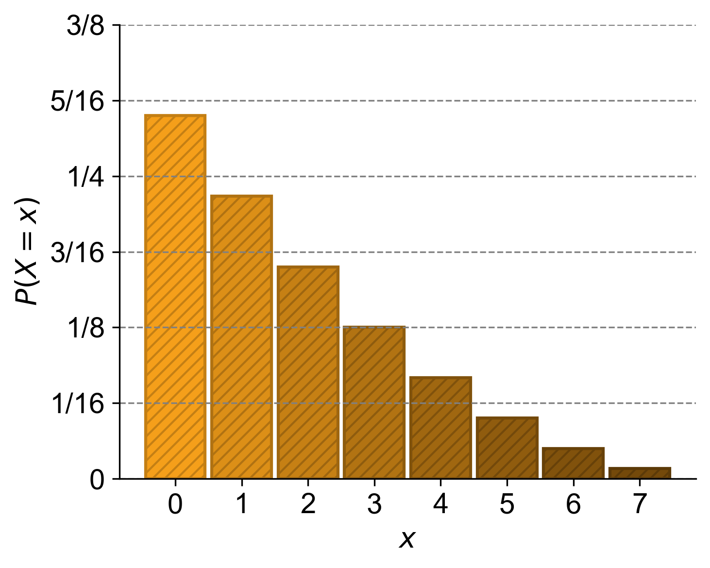
Fig. 4.4 The probability mass function (PMF) for the number of red balls picked, (W), before getting a blue one from a bag containing 10 balls (7 red and 3 blue). The random variable (W) can take values from 0 to 7.#
4.1.3. Cumulative Distribution Function (CDF)#
The Cumulative Distribution Function (CDF) of a discrete random variable \(X\) is a function that gives the probability that \(X\) will take on a value less than or equal to a certain value \(x\). It’s typically denoted as \(F_X(x)\) and is defined as:
Key properties of the CDF:
It accumulates the probabilities of the random variable from the lowest possible value up to \(x\).
For any given value \(x\), \(F_X(x)\) represents the probability that the random variable \(X\) will have a value less than or equal to \(x\).
As \(x\) increases, \(F_X(x)\) is non-decreasing (it either increases or remains constant).
\(\lim_{x \to -\infty} F_X(x) = 0\) and \(\lim_{x \to \infty} F_X(x) = 1\)
Example 4.6
Let \(X\) represent the outcome of rolling a fair six-sided die. The PMF \(p_X(x)\) would be \(\frac{1}{6}\) for \(x \in \{1, 2, 3, 4, 5, 6\}\). The CDF \(F_X(x)\) would be:
\(F_X(1) = P(X \leq 1) = \frac{1}{6}\)
\(F_X(2) = P(X \leq 2) = \frac{1}{6} + \frac{1}{6} = \frac{2}{6}\)
\(F_X(3) = P(X \leq 3) = \frac{1}{6} + \frac{1}{6} + \frac{1}{6} = \frac{3}{6}\)
… and so on, until \(F_X(6) = 1\)
The CDF is useful for finding probabilities of ranges. For example, \(P(2 < X \leq 4) = F_X(4) - F_X(2)\).
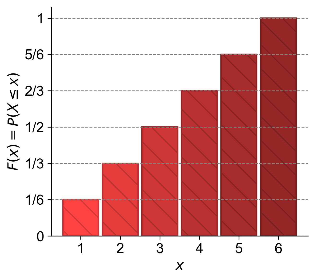
Fig. 4.5 Cumulative Distribution Function (CDF) for a Six-Sided Die. The graph illustrates the CDF for rolling a fair six-sided die. The x-axis represents the possible outcomes (1 to 6), and the y-axis shows the cumulative probability \(F_X(x)\). Each step height corresponds to the cumulative probability up to that outcome, starting from \(\frac{1}{6}\) for 1 and reaching 1 for 6.#
Summary
Probability Mass Function (PMF): The PMF of a discrete random variable \(X\) is typically denoted as \(p_X(x)\) or \(P(X = x)\). It is defined as:
(4.5)#\[\begin{equation} p_X(x) = P(X = x) \end{equation}\]This function gives the probability that the random variable \(X\) will take on the specific value \(x\). For example, if \(X\) represents the roll of a fair die, then \(p_X(3) = P(X = 3) = \frac{1}{6}\).
Cumulative Distribution Function (CDF): The CDF of \(X\), denoted as \(F_X(x)\), is defined as:
(4.6)#\[\begin{equation} F_X(x) = P(X \leq x) \end{equation}\]This function provides the probability that the random variable \(X\) will take on a value less than or equal to \(x\). It accumulates the probabilities for all outcomes up to and including \(x\).
Calculation of CDF using PMF: For a discrete random variable, the CDF \(F_X(x)\) can be calculated by summing up the PMF \(p_X(t)\) for all values \(t\) that are less than or equal to \(x\):
(4.7)#\[\begin{equation} F_X(x) = \sum_{t \leq x} p_X(t) = \sum_{t \leq x} P(X = t) \end{equation}\]This equation shows that to find \(F_X(x)\), you add up all the probabilities \(p_X(t)\) where \(t\) is any value that \(X\) could take that is also less than or equal to \(x\).
Normalization of PMF: The sum of the PMF over all possible values of \(X\) must equal 1. This is a fundamental property of probability distributions:
(4.8)#\[\begin{equation} \sum_{x} p_X(x) = \sum_{x} P(X = x) = 1 \end{equation}\]Here, the summation is over all the possible values that \(X\) can take.
Remark
It’s important to note that \( P(X = x) \) denotes the probability that the random variable \( X \) equals a specific value \( x \). However, for simplicity, in some textbooks may use the notation \( P(x) \) as shorthand for \( P(X = x) \).
Definitions - Probability Distribution
A probability distribution for a discrete random variable is a function that maps each possible value to its probability. It must satisfy the following conditions:
All probabilities are non-negative.
The sum of all probabilities is 1.
This distribution can be represented as a table, graph, or formula that lists the possible values and their associated probabilities.
Example 4.7 (Probability Analysis of a Dice Game)
Calculate the probability of each possible sum when two six-sided dice are rolled. The sum \( X \) can range from 2 to 12, and the probability \( P(X = x) \) reflects the number of ways the sum \( x \) can occur divided by the total number of possible outcomes, which is 36. For instance, there is only one way to roll a sum of 2 (1 on both dice), and there are six ways to roll a sum of 7 (1-6, 2-5, 3-4, 4-3, 5-2, 6-1).
Solution:
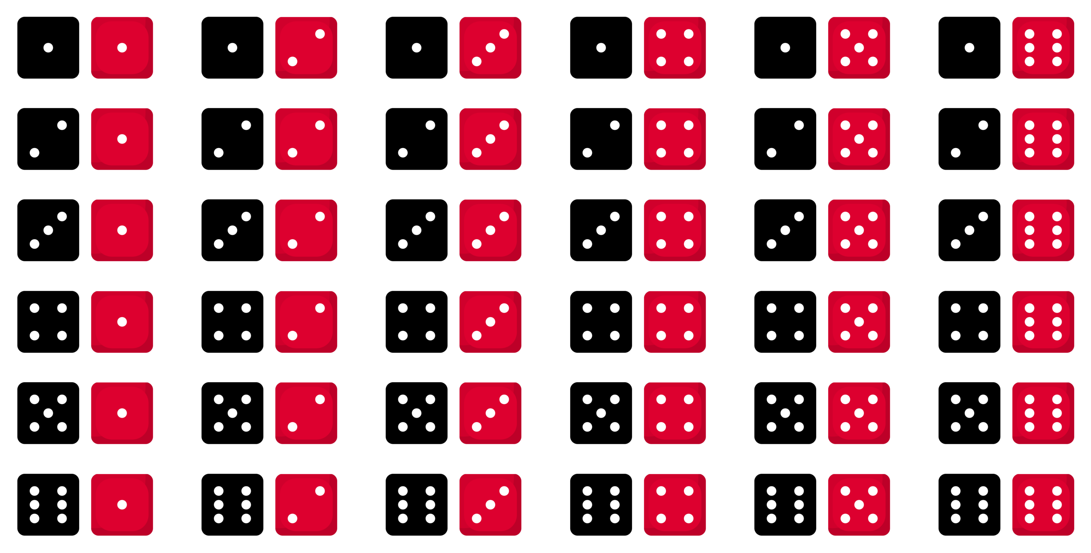
Fig. 4.6 Visualization of all possible outcomes when rolling two dice. Image based on icons from this source.#
To calculate the probabilities, we need to consider all possible combinations that can result in each sum. Here’s how we can calculate it:
Sum of 2: There is only 1 combination (1+1), so \(P(X = 2) = \frac{1}{36}\).
Sum of 3: There are 2 combinations (1+2, 2+1), so \(P(X = 3) = \frac{2}{36}\).
Sum of 4: There are 3 combinations (1+3, 2+2, 3+1), so \(P(X = 4) = \frac{3}{36}\).
Sum of 5: There are 4 combinations (1+4, 2+3, 3+2, 4+1), so \(P(X = 5) = \frac{4}{36}\).
Sum of 6: There are 5 combinations (1+5, 2+4, 3+3, 4+2, 5+1), so \(P(X = 6) = \frac{5}{36}\).
Sum of 7: There are 6 combinations (1+6, 2+5, 3+4, 4+3, 5+2, 6+1), so \(P(X = 7) = \frac{6}{36}\).
Sum of 8: There are 5 combinations (2+6, 3+5, 4+4, 5+3, 6+2), so \(P(X = 8) = \frac{5}{36}\).
Sum of 9: There are 4 combinations (3+6, 4+5, 5+4, 6+3), so \(P(X = 9) = \frac{4}{36}\).
Sum of 10: There are 3 combinations (4+6, 5+5, 6+4), so \(P(X = 10) = \frac{3}{36}\).
Sum of 11: There are 2 combinations (5+6, 6+5), so \(P(X = 11) = \frac{2}{36}\).
Sum of 12: There is only one combination (6+6), so \(P(X = 12) = \frac{1}{36}\).
These probabilities are based on the fact that each die is fair and has an equal chance of landing on any of its six faces. The total number of possible outcomes when rolling two dice is \(6 \times 6 = 36\), and each combination is equally likely.
Here’s a summary table of the probabilities:
Sum (\(X\)) |
Probability (\(P(X = x)\)) |
|---|---|
2 |
1/36 |
3 |
1/18 |
4 |
1/12 |
5 |
1/9 |
6 |
5/36 |
7 |
1/6 |
8 |
5/36 |
9 |
1/9 |
10 |
1/12 |
11 |
1/18 |
12 |
1/36 |
This table shows the probability distribution for the sum of two six-sided dice. The probabilities add up to one, as expected in a valid probability distribution.
Fig. 4.7 visually demonstrates the varying probabilities of sums when rolling two dice, highlighting that some sums, like seven, are more likely to occur than others.
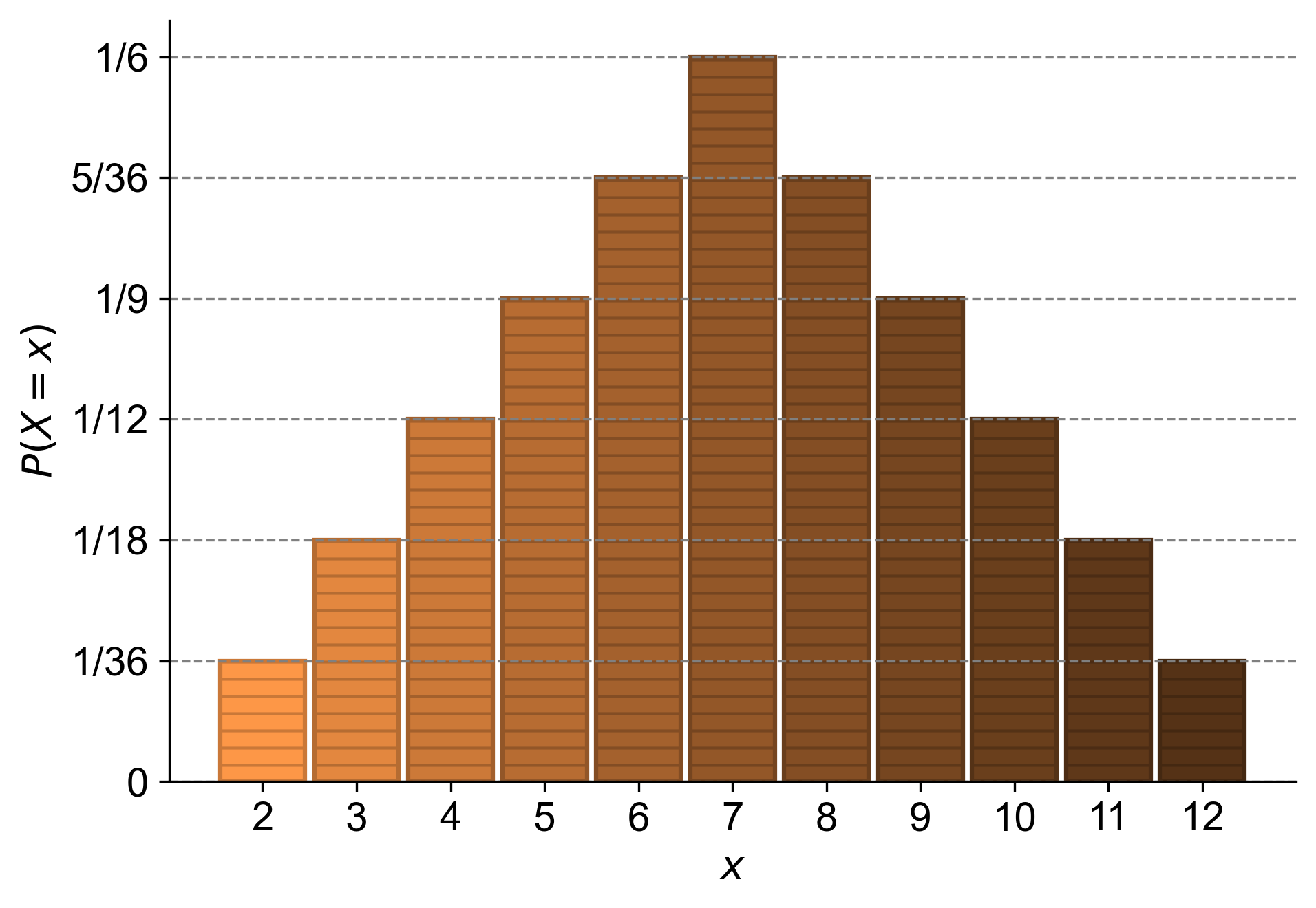
Fig. 4.7 Probability distribution graph showing that in rolling two six-sided dice, some sums occur more frequently than others; with a peak at sum seven where the probability is highest.#
Example 4.8
Given the table below, determine if the sum of the values of \( P(X = x) \) equals 1, as required for a probability distribution. Does the table describe a probability distribution?
\( x \) |
\( P(X = x) \) |
|---|---|
0 |
0.05 |
1 |
0.10 |
2 |
0.20 |
3 |
0.25 |
4 |
0.30 |
5 |
0.10 |
Solution:
\( X \) is the random variable.
The notation \( P(X = x) \) represents the probability that the random variable \( X \) takes on a specific value \( x \).
To verify if the table represents a probability distribution, we must satisfy two conditions:
The sum of the values of \( P(x) \) must equal 1.
Each value of \( P(x) \) must be non-negative (greater than or equal to 0).
Let’s evaluate both conditions for the provided table:
The sum of the values of \( P(x) \) is: \( 0.05 + 0.10 + 0.20 + 0.25 + 0.30 + 0.10 \). Calculate this sum to check if it equals 1.
Verify that each value of \( P(x) \) is non-negative.
If both conditions are met, the table represents a valid probability distribution, and the probabilities assigned to each value of \( x \) are collectively exhaustive of all possible outcomes.
Fig. 4.8 visually represents the probability distribution of a random variable (X), showing that the sum of all probabilities equals one, which is a requirement for a valid probability distribution.
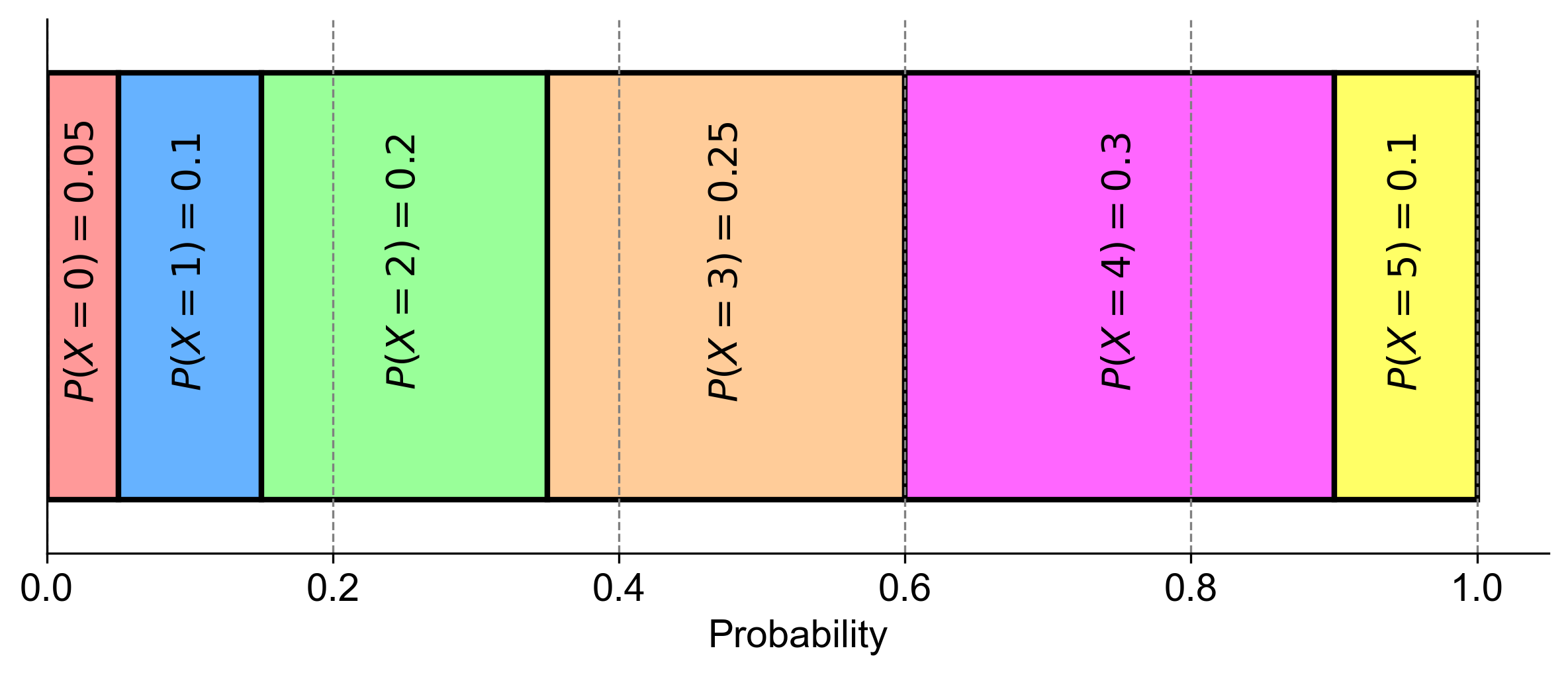
Fig. 4.8 The sum of probabilities in this discrete distribution equals one for Example 4.8.#
