4.2. Mean or Expected Value and Standard Deviation

4.2.1. Expected Value

The expected value, also known as the “long-term” average or mean, represents the average outcome we anticipate over an extended period when repeating an experiment multiple time.

For instance, consider the act of tossing a coin. The probability of getting heads on a single toss is 1/2 (assuming a fair coin), as there are two equally likely outcomes (heads or tails). However, when flipping the coin two times, probability does not dictate that we will necessarily get one heads and one tail. The outcomes of individual tosses are subject to randomness and can vary in the short term.

In contrast, probability provides insight into what can be expected over a large number of trials. For instance, if we toss a fair coin ten times, we may not always get exactly five heads and five tails. However, as the number of coin tosses increases, the actual results should converge towards the expected probability of 1/2 for heads and 1/2 for tails.

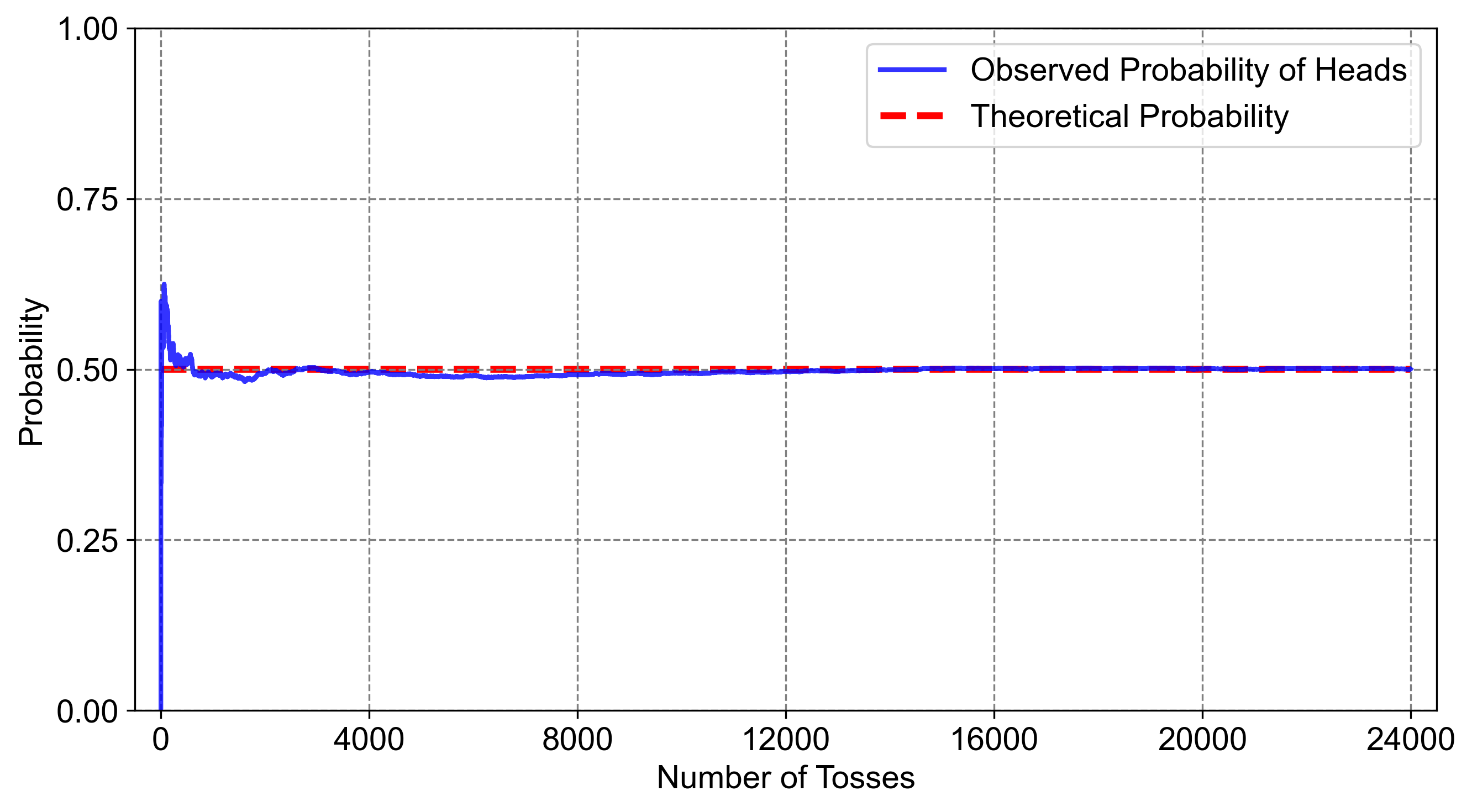
Karl Pearson’s experiment, where he tossed a fair coin 24,000 times and recorded 12,012 heads, exemplifies the Law of Large Numbers. This law states that as the number of trials in an experiment increases, the experimental results tend to converge towards the true probabilities. In Pearson’s case, the recorded percentage of heads was very close to the expected probability of 50% for a fair coin [Chang, 2012].

Fig. 4.9 illustrates the concept of expected value and the Law of Large Numbers. The blue line on the graph represents the observed probability of getting heads in a series of coin tosses. Initially, this observed probability fluctuates significantly due to the randomness inherent in short-term outcomes. In contrast, the red line represents the theoretical probability of 0.50 for heads, assuming a fair coin, and remains constant throughout.

As the number of coin tosses increases, the observed probability (blue line) gradually converges towards the theoretical probability (red line). This convergence demonstrates the Law of Large Numbers, which states that as the number of trials in an experiment increases, the experimental results tend to align more closely with the true probabilities. This graph effectively highlights how empirical evidence supports the theoretical probability over a large number of trials.

Fig. 4.9 This graph demonstrates convergence towards theoretical probability with increasing coin toss trials, highlighting empirical evidence for the Law of Large Numbers.

When examining the outcomes of statistical experiments over the long run, we often seek to understand the typical or “average” result. This long-term average, denoted by the Greek letter \(\mu\), is also known as the mean or expected value of the experiment.

In essence, the expected value represents the central tendency of the random variable under consideration. It gives us insight into the value we would anticipate on average after conducting numerous trials of the same experiment.

For example, suppose we have a random variable X that represents the results of flipping a fair coin. The possible outcomes for X are “heads” and “tails,” each with a probability of 0.5 (assuming a fair coin). The expected value (\(\mu\)) in this case would be:

\[\begin{equation*} \mu\ = \ \left\lbrack 0.5\ *\ P(heads) \right\rbrack\ + \ \left\lbrack 0.5\ *\ P(tails) \right\rbrack\ = \ 0.5\ *\ 1\ + \ 0.5\ *\ 0\ = \ 0.5 \end{equation*}\]

Thus, after performing multiple coin flips, we would expect the average proportion of heads to be approximately 0.5.

4.2.2. Mean (Expected Value) of a Discrete Random Variable

The mean of a discrete random variable X, also known as its expected value and denoted by \(E(X)\), \(\mu_X\), or simply \(\mu\), is a fundamental concept in probability theory and statistics. It represents the average value or central tendency of the random variable and is the theoretical long-term average we would expect to obtain if we repeatedly conducted the experiment or observed X multiple times.

For a discrete random variable \(X\) with potential outcomes \(x_{1}, x_{2}, \ldots, x_{n}\) and their associated probabilities \(P(X = x_{1}), P(X = x_{2}), \ldots, P(X = x_{n})\), the expected value is mathematically defined as:

(4.9)\[\begin{equation} E(X) = \mu = \sum_{i = 1}^{n} (x_i \cdot P(X = x_i)) \end{equation}\]

Where:

• \(x_i\) represents the possible values of the random variable X

• \(P(X = x_i)\) is the probability of X taking on the value \(x_i\)

Remark

1. The terms “expected value,” “expectation,” and “mean” are often used interchangeably when referring to the average value of a random variable. This measure provides insight into the central tendency of the random variable and is crucial in many areas of probability and statistics.

2. For a continuous random variable, the formula is slightly different and involves integrating over the entire range of possible values.

Example 4.9

A men’s football (also known as soccer) team engages in football activities on zero, one, or two days a week. The probabilities associated with these scenarios are as follows:

• Probability of playing zero days: 0.2

• Probability of playing one day: 0.5

• Probability of playing two days: 0.3

Determine the long-term average or expected value, \(\mu\).

Solution: Let’s define the random variable \(X\) as the number of days the men’s football team plays per week. \(X\) can take on three possible values: 0, 1, or 2.

We’ll construct a probability distribution table:

\(x\)	\(P(X = x)\)	\(x \cdot P(X = x)\)
0	0.2	0
1	0.5	0.5
2	0.3	0.6
\(\Sigma\)	1.00	1.1

The expected value can be calculated by summing up the values in the \(x * P(x)\) column:

\[\begin{equation*} \mu = E(X) = \sum_{i = 1}^{n}\left( x_i * P(X = x_i) \right) = (0)(0.2) + (1)(0.5) + (2)(0.3) = 1.1 \end{equation*}\]

Therefore, the long-term average or expected value (\(\mu\)) of the number of days per week the men’s football team plays is 1.1 days.

4.2.3. Standard Deviation of a Discrete Random Variable

The standard deviation is a crucial measure in statistics that quantifies the amount of variation or dispersion of a set of values. For a discrete random variable, it indicates how much the possible values of the variable typically deviate from the mean. A lower standard deviation implies that the values tend to be closer to the mean, while a higher standard deviation suggests they are spread out over a wider range.

Definition - Standard Deviation of a Discrete Random Variable

The standard deviation of a discrete random variable X is denoted by \(\sigma_{X}\) or, simply \(\sigma\) when no confusion will arise. It is mathematically defined as follows:

(4.10)\[\begin{equation} \sigma = \sqrt{\sum_{x} ((x - \mu)^2 \cdot P(X = x))} \end{equation}\]

In this expression, x represents the possible values of the random variable X, \(\mu\) represents the mean or expected value of X, and \(P(X = x)\) represents the probability of X taking on each specific value x.

Additionally, the standard deviation of a discrete random variable can also be computed using the alternative formula:

(4.11)\[\begin{equation} \sigma = \sqrt{\sum_{x} (x^2 \cdot P(X = x)) - \mu^2} \end{equation}\]

This formula calculates the standard deviation by summing the squared values of X, each multiplied by its respective probability, and then subtracting the square of the mean.

Note

It’s worth noting that the variance, which is the square of the standard deviation, can be expressed as:

(4.12)\[\begin{equation}\sigma^2 = E(X^2) - (E(X))^2\end{equation}\]

This formula relates the variance to the expected value of X squared and the square of the expected value of X, providing an alternative way to conceptualize and calculate the variance and standard deviation.

Example 4.10

In a small town, the random variable \(Y\) represents the number of power outages occurring in a year. The probabilities of having 0, 1, 2, 3, or 4 power outages are given in the table below. Determine whether this table represents a probability distribution. If it does, calculate its mean and standard deviation.

\(y\)	\(P(Y = y)\)
0	0.05
1	0.20
2	0.40
3	0.25
4	0.10

Solution: First, we check if the sum of the probabilities equals 1:

\[\begin{equation*} \sum P(Y = y) = 0.05 + 0.20 + 0.40 + 0.25 + 0.10 = 1.00 \end{equation*}\]

Since the sum is 1, the first condition for a probability distribution is satisfied.

Next, we check if all probabilities are non-negative:

All given probabilities are greater than or equal to 0, so the second condition is also satisfied.

Thus, the table represents a valid probability distribution.

Now, let’s calculate the mean (\(\mu\)):

\[\begin{equation*} \mu = E(Y) = \sum y \cdot P(Y = y) = 0 \cdot 0.05 + 1 \cdot 0.20 + 2 \cdot 0.40 + 3 \cdot 0.25 + 4 \cdot 0.10 = 2.15 \end{equation*}\]

Finally, we calculate the standard deviation (\(\sigma\)) using two approaches:

Approach 1: Using the definition formula

\[\begin{align*} \sigma &= \sqrt{\sum (y - \mu)^2 \cdot P(Y = y)}\\ &= \sqrt{(0 - 2.15)^2 \cdot 0.05 + (1 - 2.15)^2 \cdot 0.20 + (2 - 2.15)^2 \cdot 0.40 + (3 - 2.15)^2 \cdot 0.25 + (4 - 2.15)^2 \cdot 0.10}\\ &= \sqrt{4.6225 \cdot 0.05 + 1.3225 \cdot 0.20 + 0.0225 \cdot 0.40 + 0.7225 \cdot 0.25 + 3.4225 \cdot 0.10}\\ &= \sqrt{0.2311125 + 0.26450 + 0.0090 + 0.180625 + 0.34225}\\ &= \sqrt{1.0275} \approx 1.0137 \end{align*}\]

Approach 2: Using \(\sigma^2 = E(Y^2) - (E(Y))^2\)

First, calculate \(E(Y^2)\):

\[\begin{align*} E(Y^2) &= \sum y^2 \cdot P(Y = y)\\ &= 0^2 \cdot 0.05 + 1^2 \cdot 0.20 + 2^2 \cdot 0.40 + 3^2 \cdot 0.25 + 4^2 \cdot 0.10\\ &= 0 + 0.20 + 1.60 + 2.25 + 1.60 = 5.65 \end{align*}\]

Now, calculate \(\sigma^2\):

\[\begin{align*} \sigma^2 &= E(Y^2) - (E(Y))^2\\ &= 5.65 - 2.15^2\\ &= 5.65 - 4.6225 = 1.0275 \end{align*}\]

Therefore, \(\sigma = \sqrt{1.0275} \approx 1.0137\)

Both approaches yield the same result: The mean number of power outages in the town is 2.15 per year, with a standard deviation of approximately 1.0137.

Note

We can also calculate \(\sigma^2\) using a tabular approach with the formula \(\sigma^2 = E(Y^2) - (E(Y))^2\). Let’s create a table with columns for \(y\), \(P(Y = y)\), \(y \cdot P(Y = y)\), and \(y^2 \cdot P(Y = y)\):

\(y\)	\(P(Y = y)\)	\(y \cdot P(Y = y)\)	\(y^2 \cdot P(Y = y)\)
0	0.05	0	0
1	0.2	0.2	0.2
2	0.4	0.8	1.6
3	0.25	0.75	2.25
4	0.1	0.4	1.6
\(\Sigma\)	1.00	2.15	5.65

From this table:

\[\begin{align*} E(Y) &= \sum(y \cdot P(Y = y)) = 2.15 \\ E(Y^2) &= \sum(y^2 \cdot P(Y = y)) = 5.65 \end{align*}\]

Now we can calculate \(\sigma^2\):

\[\begin{equation*} \sigma^2 = E(Y^2) - (E(Y))^2 = 5.65 - 2.15^2 = 5.65 - 4.6225 = 1.0275 \end{equation*}\]

Therefore, \(\sigma = \sqrt{1.0275} \approx 1.0137\), which matches our previous calculations.

Example 4.11

A local bakery is analyzing the number of loaves of bread sold each day. The random variable \(Z\) represents the number of loaves sold. Based on past sales data, the probabilities for selling 0, 1, 2, 3, or 4 loaves are given in the table below. Determine if this table represents a probability distribution. If it does, calculate its mean and standard deviation.

\(z\)	\(P(Z = z)\)
0	0.10
1	0.15
2	0.25
3	0.30
4	0.20

Solution: First, we check if the sum of the probabilities equals 1:

\[\begin{equation*} \sum P(Z = z) = 0.10 + 0.15 + 0.25 + 0.30 + 0.20 = 1.00 \end{equation*}\]

Since the sum is 1, the first condition for a probability distribution is satisfied.

Next, we check if all probabilities are non-negative:

All given probabilities are greater than or equal to 0, so the second condition is also satisfied.

Thus, the table represents a valid probability distribution.

Now, let’s calculate the mean (\(\mu\)):

\[\begin{equation*} \mu = E(Z) = \sum z \cdot P(Z = z) = 0 \cdot 0.10 + 1 \cdot 0.15 + 2 \cdot 0.25 + 3 \cdot 0.30 + 4 \cdot 0.20 = 2.35 \end{equation*}\]

Finally, we calculate the standard deviation (\(\sigma\)) using two approaches:

Approach 1: Using the definition formula

\[\begin{align*} \sigma &= \sqrt{\sum (z - \mu)^2 \cdot P(Z = z)}\\ &= \sqrt{(0 - 2.35)^2 \cdot 0.10 + (1 - 2.35)^2 \cdot 0.15 + (2 - 2.35)^2 \cdot 0.25 + (3 - 2.35)^2 \cdot 0.30 + (4 - 2.35)^2 \cdot 0.20}\\ &= \sqrt{5.5225 \cdot 0.10 + 1.8225 \cdot 0.15 + 0.1225 \cdot 0.25 + 0.4225 \cdot 0.30 + 2.7225 \cdot 0.20}\\ &= \sqrt{0.55225 + 0.273375 + 0.030625 + 0.126750 + 0.544500}\\ &= \sqrt{1.530475} \approx 1.2359 \end{align*}\]

Approach 2: Using \(\sigma^2 = E(Z^2) - (E(Z))^2\)

First, calculate \(E(Z^2)\):

\[\begin{align*} E(Z^2) &= \sum z^2 \cdot P(Z = z)\\ &= 0^2 \cdot 0.10 + 1^2 \cdot 0.15 + 2^2 \cdot 0.25 + 3^2 \cdot 0.30 + 4^2 \cdot 0.20\\ &= 0 + 0.15 + 1.00 + 2.70 + 3.20 = 7.05 \end{align*}\]

Now, calculate \(\sigma^2\):

\[\begin{align*} \sigma^2 &= E(Z^2) - (E(Z))^2\\ &= 7.05 - 2.35^2\\ &= 7.05 - 5.5225 = 1.5275 \end{align*}\]

Therefore, \(\sigma = \sqrt{1.5275} \approx 1.2359\)

Both approaches yield the same result: The mean number of loaves sold by the bakery is 2.35 per day, with a standard deviation of approximately 1.2359.

Note

We can also calculate \(\sigma^2\) using a tabular approach with the formula \(\sigma^2 = E(Z^2) - (E(Z))^2\). Let’s create a table with columns for \(z\), \(P(Z = z)\), \(z \cdot P(Z = z)\), and \(z^2 \cdot P(Z = z)\):

\(z\)	\(P(Z = z)\)	\(z \cdot P(Z = z)\)	\(z^2 \cdot P(Z = z)\)
0	0.10	0	0
1	0.15	0.15	0.15
2	0.25	0.50	1.00
3	0.30	0.90	2.70
4	0.20	0.80	3.20
\(\Sigma\)	1.00	2.35	7.05

From this table:

\[\begin{align*} E(Z) &= \sum(z \cdot P(Z = z)) = 2.35\\ E(Z^2) &= \sum(z^2 \cdot P(Z = z)) = 7.05\\ \end{align*}\]

Now we can calculate \(\sigma^2\):

\[\begin{equation*}\sigma^2 = E(Z^2) - (E(Z))^2 = 7.05 - 2.35^2 = 7.05 - 5.5225 = 1.5275\end{equation*}\]

Therefore, \(\sigma = \sqrt{1.5275} \approx 1.2359\), which matches our previous calculations.

Example 4.12

A survey was conducted to determine the favorite fruit of students in a school. The random variable \(W\) represents the number of students choosing a particular fruit. The probabilities for choosing an apple, banana, cherry, date, or elderberry are given in the table below.

• a. Determine if this table represents a probability distribution.

• b. If it does, calculate its mean.

• c. Calculate the standard deviation.

Fruit (\(W\))	\(P(W)\)
Apple (1)	0.30
Banana (2)	0.25
Cherry (3)	0.20
Date (4)	0.15
Elderberry (5)	0.10

Solution:

a. To determine if this is a probability distribution:

First, we check if the sum of the probabilities equals 1:

\[\begin{equation*} \sum P(W) = 0.30 + 0.25 + 0.20 + 0.15 + 0.10 = 1.00 \end{equation*}\]

Since the sum is 1, the first condition for a probability distribution is satisfied.

Next, we check if all probabilities are non-negative: All given probabilities are greater than or equal to 0, so the second condition is also satisfied.

Thus, the table represents a valid probability distribution.

b. To calculate the mean (\(\mu\)):

The mean (\(\mu\)) is calculated as:

\[\begin{equation*} \mu = E(W) = \sum W \cdot P(W) = 1 \cdot 0.30 + 2 \cdot 0.25 + 3 \cdot 0.20 + 4 \cdot 0.15 + 5 \cdot 0.10 = 2.50 \end{equation*}\]

c. To calculate the standard deviation (\(\sigma\)):

Approach 1: Using the definition formula

\[\begin{align*} \sigma &= \sqrt{\sum (W - \mu)^2 \cdot P(W)} \\ &= \sqrt{(1 - 2.50)^2 \cdot 0.30 + (2 - 2.50)^2 \cdot 0.25 + (3 - 2.50)^2 \cdot 0.20 + (4 - 2.50)^2 \cdot 0.15 + (5 - 2.50)^2 \cdot 0.10} \\ &= \sqrt{2.25 \cdot 0.30 + 0.25 \cdot 0.25 + 0.25 \cdot 0.20 + 2.25 \cdot 0.15 + 6.25 \cdot 0.10} \\ &= \sqrt{0.675 + 0.0625 + 0.05 + 0.3375 + 0.625} \\ &= \sqrt{1.75} \approx 1.3229 \end{align*}\]

Approach 2: Using \(\sigma^2 = E(W^2) - (E(W))^2\)

First, calculate \(E(W^2)\):

\[\begin{align*} E(W^2) &= \sum W^2 \cdot P(W)\\ &= 1^2 \cdot 0.30 + 2^2 \cdot 0.25 + 3^2 \cdot 0.20 + 4^2 \cdot 0.15 + 5^2 \cdot 0.10\\ &= 0.30 + 1.00 + 1.80 + 2.40 + 2.50 = 8.00 \end{align*}\]

Now, calculate \(\sigma^2\):

\[\begin{align*} \sigma^2 &= E(W^2) - (E(W))^2\\ &= 8.00 - 2.50^2\\ &= 8.00 - 6.25 = 1.75 \end{align*}\]

Therefore, \(\sigma = \sqrt{1.75} \approx 1.3229\)

Both approaches yield the same result: The mean favorite fruit ranking is 2.50 with a standard deviation of approximately 1.3229.

Note

We can also calculate \(\sigma^2\) using a tabular approach with the formula \(\sigma^2 = E(W^2) - (E(W))^2\). Let’s create a table with columns for \(w\), \(P(W = w)\), \(w \cdot P(W = w)\), and \(w^2 \cdot P(W = w)\):

\(w\)	\(P(W = w)\)	\(w \cdot P(W = w)\)	\(w^2 \cdot P(W = w)\)
1	0.30	0.30	0.30
2	0.25	0.50	1.00
3	0.20	0.60	1.80
4	0.15	0.60	2.40
5	0.10	0.50	2.50
\(\Sigma\)	1.00	2.50	8.00

From this table:

\[\begin{align*} E(W) &= \sum(w \cdot P(W = w)) = 2.50\\ E(W^2) &= \sum(w^2 \cdot P(W = w)) = 8.00\\ \end{align*}\]

Now we can calculate \(\sigma^2\):

\[\begin{equation*}\sigma^2 = E(W^2) - (E(W))^2 = 8.00 - 2.50^2 = 8.00 - 6.25 = 1.75\end{equation*}\]

Therefore, \(\sigma = \sqrt{1.75} \approx 1.3229\), which matches our previous calculations.

This tabular approach provides a clear and organized method for calculating the variance and standard deviation, especially useful for more complex probability distributions.

Understanding Cumulative Probabilities Through Visual Aids

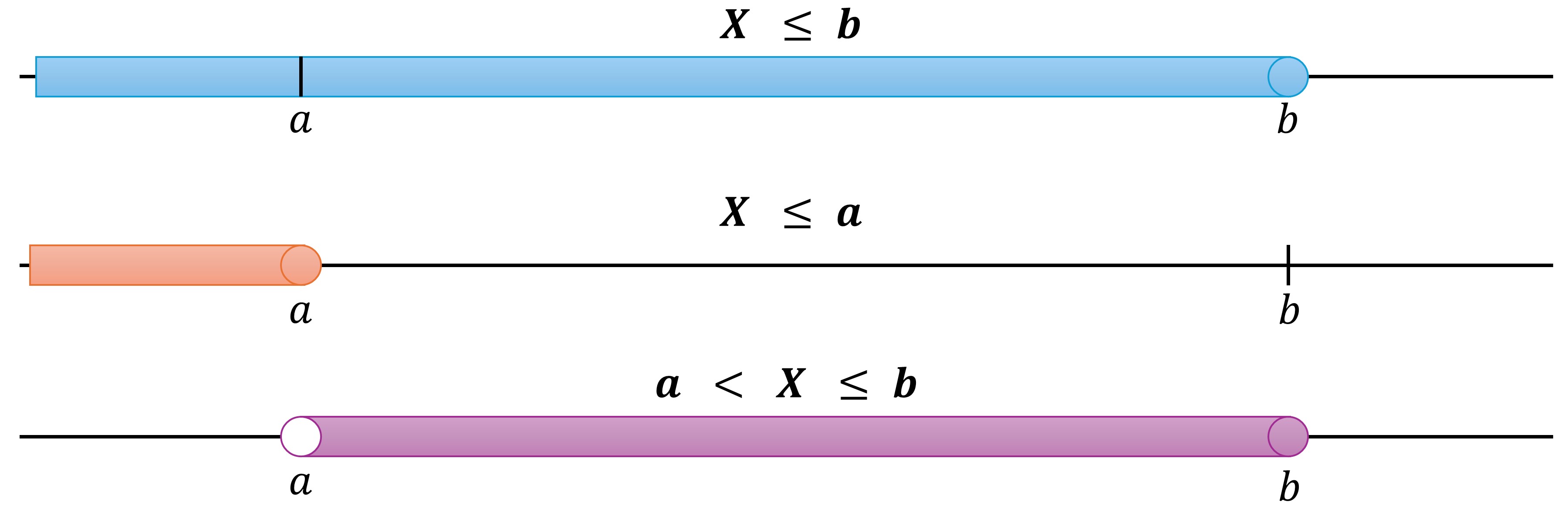
Cumulative probability represents the likelihood that a random variable is less than or equal to a specified value, denoted as \(P(X \leq x)\). This concept is particularly useful when determining the probability of a random variable falling within a specific range. We can express this probability using two slightly different formulations:

1. For an exclusive lower bound and inclusive upper bound:

   \[\begin{equation*} P(a < X \leq b) = P(X \leq b) - P(X \leq a) \end{equation*}\]

   In this case, we’re calculating the probability that \(X\) falls strictly above \(a\) and up to and including \(b\). This is done by subtracting the cumulative probability up to \(a\) from the cumulative probability up to \(b\). The result gives us the probability in the interval \((a, b]\).

   

   Fig. 4.10 Probability Range for \(a < X \leq b\): The purple area illustrates the probability of X falling between \(a\) (exclusive) and \(b\) (inclusive). The blue area represents \(P(X \leq b)\), while the orange area shows \(P(X \leq a)\). The difference between these areas (purple) is \(P(a < X \leq b)\).

2. For an inclusive lower bound and inclusive upper bound:

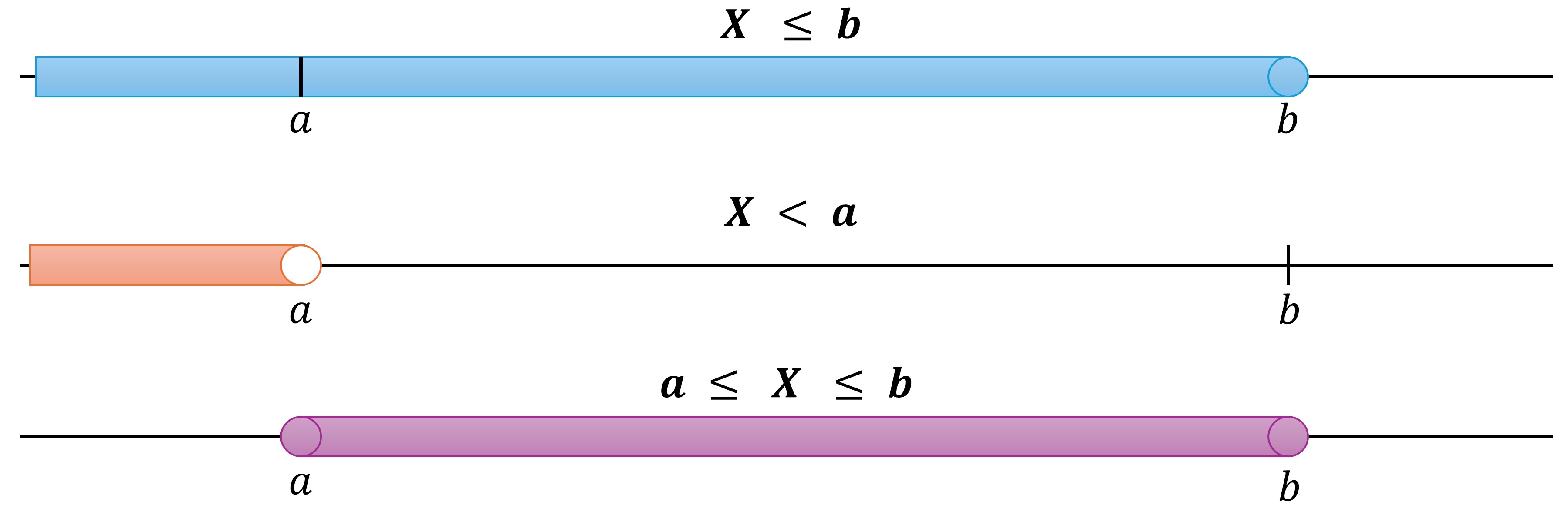
   \[\begin{equation*} P(a \leq X \leq b) = P(X \leq b) - P(X < a) \end{equation*}\]

   Here, we’re calculating the probability that \(X\) falls in the closed interval \([a, b]\). This is achieved by subtracting the cumulative probability strictly less than a from the cumulative probability up to and including \(b\). This formulation ensures that the probability at exactly \(a\) is included in our calculation.

   

   Fig. 4.11 Probability Range for \(a \leq X \leq b\): The purple area demonstrates the probability of X falling between \(a\) and \(b\), both inclusive. Here, the blue area represents \(P(X \leq b)\), and the orange area represents \(P(X < a)\). The purple area, their difference, shows \(P(a \leq X \leq b)\).

Fig. 4.10 and Fig. 4.11 effectively illustrate how cumulative probabilities can be utilized to calculate the probability of a random variable within specific intervals. The key difference between the two figures lies in the treatment of the lower bound: exclusive in the first case and inclusive in the second.

Example 4.13

A company is conducting quality control tests on the light bulbs they manufacture. The random variable \(Y\) represents the number of defective light bulbs found in a sample of six. The probabilities for each number of defective bulbs are given in the table below. Answer the following questions based on the table.

Number of Defective Bulbs (\(Y\))	\(P(Y = y)\)
0	0.40
1	0.35
2	0.15
3	0.05
4	0.04
5	0.01
6	0.00

• a. Find the probability of finding exactly 1 defective light bulb.

• b. Find the probability of finding 2 or more defective light bulbs.

• c. Find the probability of finding no defective light bulbs.

• d. Find the probability of finding 3 or fewer defective light bulbs.

Solution:

a. The probability of finding exactly 1 defective light bulb is \( P(Y = 1) = 0.35 \).

b. The probability of finding 2 or more defective light bulbs is the sum of the probabilities of finding 2, 3, 4, 5, and 6 defective bulbs:

\[\begin{equation*} P(Y \geq 2) = P(Y = 2) + P(Y = 3) + P(Y = 4) + P(Y = 5) + P(Y = 6) = 0.15 + 0.05 + 0.04 + 0.01 + 0.00 = 0.25 \end{equation*}\]

c. The probability of finding no defective light bulbs is \( P(Y = 0) = 0.40 \).

d. The probability of finding 3 or fewer defective light bulbs is the sum of the probabilities of finding 0, 1, 2, or 3 defective bulbs:

\[\begin{equation*} P(Y \leq 3) = P(Y = 0) + P(Y = 1) + P(Y = 2) + P(Y = 3) = 0.40 + 0.35 + 0.15 + 0.05 = 0.95 \end{equation*}\]

Example 4.14

A manufacturer specifies that a light bulb should have a lifespan in the range of 900–1100 hours. A quality control engineer tests two light bulbs. The probabilities are given as follows:

• Both light bulbs meet the lifespan specification: 0.25

• Exactly one light bulb meets the specification: 0.50

• Neither light bulb meets the specification: 0.25

Let Y represent the number of light bulbs that meet the lifespan specification.

• a) Determine the probability mass function (PMF) of Y.

• b) Calculate the mean of Y.

• c) Calculate the variance of Y.

• d) Calculate the standard deviation of Y.

Solution:

a) Probability Mass Function (PMF) of Y:

The PMF of Y is defined as:

• \(P(Y = 0) = 0.25\) (neither bulb meets specification)

• \(P(Y = 1) = 0.50\) (exactly one bulb meets specification)

• \(P(Y = 2) = 0.25\) (both bulbs meet specification)

• \(P(Y = y) = 0\) for \(y \neq 0, 1, 2\)

b) Mean (\(\mu_Y\)) of Y:

The mean is calculated as:

\[\begin{align*} \mu_Y &= \sum y \cdot P(Y = y) \\ &= (0 \cdot 0.25) + (1 \cdot 0.50) + (2 \cdot 0.25) \\ &= 0 + 0.50 + 0.50 \\ &= 1.00 \end{align*}\]

c) Variance (\(\sigma^2_Y\)) of Y:

To find the variance, we first calculate \(E(Y^2)\):

\[\begin{align*} E(Y^2) &= \sum y^2 \cdot P(Y = y) \\ &= (0^2 \cdot 0.25) + (1^2 \cdot 0.50) + (2^2 \cdot 0.25) \\ &= 0 + 0.50 + 1.00 \\ &= 1.50 \end{align*}\]

Now, we can calculate the variance:

\[\begin{align*} \sigma^2_Y &= E(Y^2) - (\mu_Y)^2 \\ &= 1.50 - (1.00)^2 \\ &= 1.50 - 1.00 \\ &= 0.50 \end{align*}\]

d) Standard Deviation (\(\sigma_Y\)) of Y:

The standard deviation is the square root of the variance:

\[\begin{align*} \sigma_Y &= \sqrt{\sigma^2_Y} \\ &= \sqrt{0.50} \\ &\approx 0.7071 \end{align*}\]

Example 4.15

A game show offers contestants the chance to win a prize by spinning a wheel with 10 equal sections, numbered 1 through 10. The contestant wins if the wheel stops on any number from 1 to 5. If the contestant spins the wheel twice, calculate the following:

• a. The probability mass function for the number of times the contestant wins.

• b. The mean number of wins.

• c. The variance and standard deviation of the number of wins.

Solution: Let \(Z\) represent the number of times the contestant wins. The possible values of \(Z\) are 0, 1, or 2.

a. Probability Mass Function (PMF): The probability of winning on a single spin is 5/10 = 0.5. Using this, we can calculate:

• \(P(Z = 0)\): Probability of losing both spins = \((0.5)^2 = 0.25\)

• \(P(Z = 1)\): Probability of winning exactly one spin = \(2(0.5)(0.5) = 0.50\)

• \(P(Z = 2)\): Probability of winning both spins = \((0.5)^2 = 0.25\)

We can verify this is a valid probability distribution:

• Sum of probabilities: 0.25 + 0.50 + 0.25 = 1.0

• All probabilities are non-negative Therefore, this is a valid probability distribution.

b. Mean (\(\mu_Z\)): The mean number of wins is calculated as:

\[\mu_Z = 0(0.25) + 1(0.50) + 2(0.25) = 1.00\]

On average, the contestant is expected to win once in two spins.

c. Variance (\(\sigma^2_Z\)) and Standard Deviation (\(\sigma_Z\)): To calculate the variance, we first need \(E(Z^2)\):

\[E(Z^2) = 0^2(0.25) + 1^2(0.50) + 2^2(0.25) = 1.50\]

Now we can calculate the variance:

\[\sigma^2_Z = E(Z^2) - (\mu_Z)^2 = 1.50 - (1.00)^2 = 0.50\]

The standard deviation is the square root of the variance:

\[\sigma_Z = \sqrt{\sigma^2_Z} = \sqrt{0.50} \approx 0.7071\]

This standard deviation indicates the typical deviation from the mean number of wins.

Table 4.1 provides a comprehensive list of mathematical symbols, their verbal equivalents, and their opposites. It can be used as a reference for understanding and communicating mathematical relationships in verbal form.

Table 4.1 Comprehensive Reference of Mathematical Symbols and Their Verbal Interpretations

Symbol	Verbal Equivalent	Opposite Symbol	Opposite Verbal Equivalent
\( > \)	Is greater than	\( < \)	Is less than
\( > \)	Is above	\( < \)	Is below
\( > \)	Is higher than	\( < \)	Is lower than
\( > \)	Is longer than	\( < \)	Is shorter than
\( > \)	Is bigger than	\( < \)	Is smaller than
\( > \)	Is more than	\( < \)	Is fewer than
\( > \)	Is increased from	\( < \)	Is decreased from
\( \geq \)	Is greater than or equal to	\( \leq \)	Is less than or equal to
\( \geq \)	Is at least	\( \leq \)	Is at most
\( \geq \)	Is no less than	\( \leq \)	Is no more than
\( = \)	Is equal to	\( \neq \)	Is not equal to
\( = \)	Is equivalent to	\( \neq \)	Is not equivalent to
\( = \)	Is identical to	\( \neq \)	Is not identical to
\( = \)	Is the same as	\( \neq \)	Is different from
\( = \)	Has not changed from	\( \neq \)	Has changed from