2.8. Measures of Variation

2.8.1. Measures of Variation or Spread in Soccer Player Heights

Consider an example involving the heights of five starting players from two soccer teams. Both teams share the same average height, which is approximately 180 centimeters (equivalent to 5’11”). Additionally, they have the same middle height value, known as the median, which is approximately 183 centimeters (equivalent to 6’0”). Despite these similarities, there are notable differences between the two sets of data. Specifically, the heights of the players on Team II exhibit much more variability compared to Team I.

To quantitatively describe this difference in variation, we use descriptive measures, often referred to as measures of variation or spread. Just as there are various measures of central tendency, there are also several measures of variation. In this context, we will focus on two commonly used measures:

1. Range: The range represents the difference between the tallest and shortest player’s height in a dataset. It provides a simple measure of how spread out the data points are. For our soccer player heights, the range would be the difference between the tallest and shortest player.

2. Sample Standard Deviation: The sample standard deviation measures the average deviation of individual data points from the mean (average). It quantifies the spread of data around the mean. A larger standard deviation indicates greater variability. For our heights example, calculating the sample standard deviation would reveal how much the heights deviate from the average.

Other terms synonymous with dispersion include spread and scatter.

Definition - Range of a Data Set

The range of a data set represents the spread or variability of the observations. It is calculated as the difference between the maximum and minimum values in the data set.

Mathematically, the range can be expressed using the following formula:

(2.20)\[\begin{equation} \text{Range} = \text{Max} - \text{Min} \end{equation}\]

Where:

• \(\text{Max}\) represents the maximum observation in the data set.

• \(\text{Min}\) represents the minimum observation in the data set.

Example 2.52 (Soccer Player Heights)

We’re comparing the heights of soccer players from two different teams to understand how much variation there is in player heights within each team.

• Team I:

  • The tallest player is 190 centimeters tall.

  • The shortest player is 175 centimeters tall.

  • To find the range, we subtract the shortest player’s height from the tallest player’s height:

  \[\begin{equation*}\text{Range for Team I} = 190 \text{ cm} - 175 \text{ cm} = 15 \text{ cm}\end{equation*}\]

This means that all the players on Team I have heights that fall within a 15-centimeter span. There’s less variability in their heights, indicating that the players are more similar in stature.

• Team II:

  • The tallest player is 195 centimeters tall.

  • The shortest player is 160 centimeters tall.

  • Similarly, we find the range for Team II:

  \[\begin{equation*}\text{Range for Team II} = 195 \text{ cm} - 160 \text{ cm} = 35 \text{ cm}\end{equation*}\]

Here, the players on Team II have heights that span a 35-centimeter range. This is a larger range than Team I, showing that there’s greater variability in the heights of Team II’s players. They vary more in height, from quite short to very tall.

The range tells us about the spread of heights within each team. Team II has a greater range, meaning its players’ heights are more varied compared to Team I, where players have more similar heights. This can be useful information for understanding the physical diversity of a team.

Definition - Sum of Squared Deviations (SSD)

The Sum of Squared Deviations is a measure that quantifies how much individual data points deviate from the mean (average) of a dataset. It helps us understand the overall variability or spread within the data.

Mathematically, the SSD can be calculated as follows:

(2.21)\[\begin{equation} \text{SSD} = \sum_{i=1}^{n} (x_i - \bar{x})^2 \end{equation}\]

Where:

• \(n\) represents the total number of data points (in our case, the number of football players).

• \(x_i\) represents the height of the \(i\)-th football player.

• \(\bar{x}\) represents the mean height of all the players.

Example 2.53 (Heights of 11 Football Players)

The heights (in cm) for 11 football players are as follows:

\[\begin{equation*}\text{Player Heights} = [180, 185, 175, 190, 170, 182, 188, 176, 183, 178, 184]\end{equation*}\]

• a. Calculate the range of the players’ height.

• b. Calculate the mean height of the players.

• c. Compute the squared deviations from the mean for each player.

• d. Sum up the squared deviations to find the total squared deviation (SSD).

Solution:

a. Range of the Players’ Height Calculation:

\[\begin{equation*}\text{Range for Players' Heights} = 190 \text{ cm} - 170 \text{ cm} = 20 \text{ cm}\end{equation*}\]

Fig. 2.62 Visualizing the Range of Player Heights for Example 2.53.

b. Mean Height Calculation: The mean height (\(\bar{x}\)) is the average height of all players. It is calculated by summing all the heights and dividing by the number of players.

\[\begin{align*} \bar{x} &= \dfrac{\sum \text{heights}}{\text{number of players}} \\ &= \dfrac{180 + 185 + 175 + 190 + 170 + 182 + 188 + 176 + 183 + 178 + 184}{11} \\ &= 181 \text{ cm} \end{align*}\]

c. Squared Deviations: The squared deviation for each player is the square of the difference between that player’s height and the mean height.

• For the first player: \((180 - 181)^2 = 1\)

• This process is repeated for each player to find their individual squared deviations.

d. Sum of Squared Deviations (SSD): The SSD is the sum of all squared deviations, providing insight into the variability of heights.

\[\begin{equation*}\text{SSD} = \sum (x - \bar{x})^2 = 1 + 16 + 36 + 81 + 121 + 1 + 49 + 25 + 4 + 9 + 9 = 352\end{equation*}\]

The mean height is a central value that gives us a reference point to compare individual heights. The deviations tell us how far each player’s height is from this average. By squaring these deviations, we emphasize larger differences and eliminate negative values, making it easier to aggregate them. The SSD then sums these squared deviations to give a single measure of overall variability. In sports science, understanding this variability can help in designing training programs and strategies that cater to the physical diversity within a team.

Player Number	Height x	Deviation \((x - \bar{x})\)	Squared Deviation \((x - \bar{x})^2\)
1	180	-1	1
2	185	4	16
3	175	-6	36
4	190	9	81
5	170	-11	121
6	182	1	1
7	188	7	49
8	176	-5	25
9	183	2	4
10	178	-3	9
11	184	3	9
		Total SSD	352

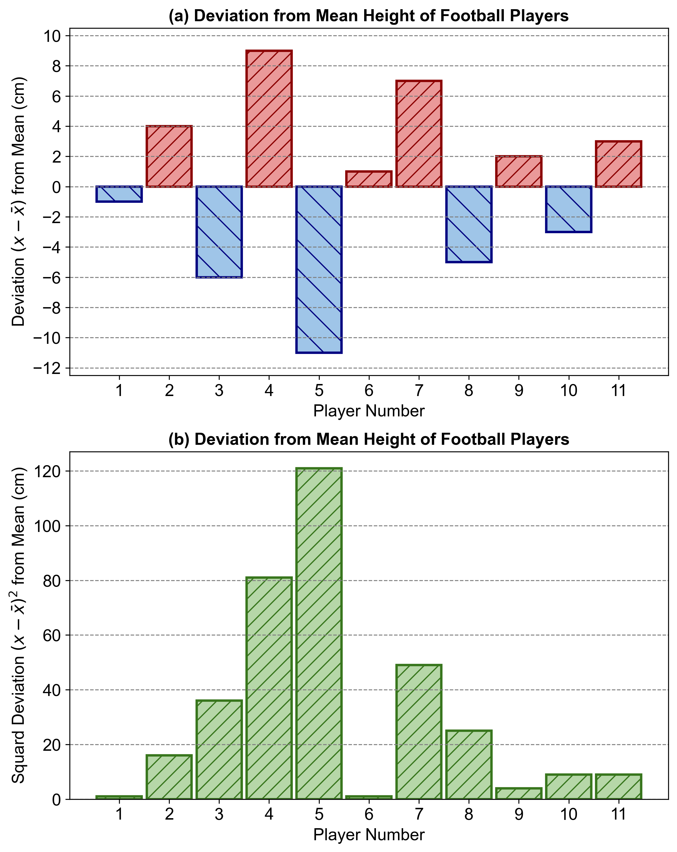
This table helps visualize the calculation process and the resulting SSD, which is crucial for understanding the team’s physical composition.

Fig. 2.63 (a): Deviation from Mean Height of Football Players. (b): Squared Deviation from Mean Height of Football Players.

2.8.2. Sample Variance and Standard Deviation

After calculating the squared deviations, the subsequent step in computing a sample standard deviation involves finding the average of these squared deviations. To achieve this, we divide the sum of squared deviations by \(n - 1\), where \(n\) represents the sample size. The resulting value is referred to as the sample variance and is denoted as \(s_x^2\) or simply \(s^2\) when there is no possibility of confusion. Symbolically, this can be expressed as follows:

(2.22)\[\begin{equation} s^2 = \dfrac{1}{n - 1}\sum_{i=1}^{n} (x_i - \bar{x})^2 \end{equation}\]

Definition - Sample Variance

The sample variance is a statistical measure that quantifies the spread or variability of data points within a sample. It provides insight into how individual data values deviate from the sample mean (average).

Mathematically, the sample variance (\(s^2\)) is calculated as follows:

(2.23)\[\begin{equation} s^2 = \dfrac{1}{n - 1}\sum_{i=1}^{n} (x_i - \bar{x})^2 \end{equation}\]

Where:

• \(n\) represents the sample size (number of data points).

• \(x_i\) represents the individual data value.

• \(\bar{x}\) represents the sample mean (average).

• Steps to Calculate Sample Variance:

  1. Compute the Sample Mean:

     • Add up all the data values and divide by the sample size:

       (2.24)\[\begin{equation} \bar{x} = \dfrac{1}{n} \sum_{i=1}^{n} x_i \end{equation}\]

  2. Calculate the Squared Deviations:

     • For each data value, subtract the sample mean and square the result:

       (2.25)\[\begin{equation} (x_i - \bar{x})^2 \end{equation}\]

  3. Sum Up the Squared Deviations:

     • Add all the squared deviations together:

       (2.26)\[\begin{equation} \sum_{i=1}^{n} (x_i - \bar{x})^2 \end{equation}\]

  4. Divide by \(n - 1\):

     • Divide the sum of squared deviations by \(n - 1\) to account for the degrees of freedom (adjustment for sample size):

       (2.27)\[\begin{equation} s^2 = \dfrac{1}{n - 1} \sum_{i=1}^{n} (x_i - \bar{x})^2 \end{equation}\]

• Interpretation:

  • A larger sample variance indicates greater variability among data points.

  • The sample variance is measured in units that are the square of the original data units.

Note

Degrees of Freedom (df): In statistics, degrees of freedom refer to the number of independent values or quantities that can vary in an analysis without breaking any constraints. It is a fundamental concept that appears in various statistical calculations, where it often determines the shape of different sampling distributions.

For the calculation of sample variance, the degrees of freedom are defined as the sample size minus one (\( n - 1 \)). This subtraction accounts for the fact that we are using the sample mean (\( \bar{x} \)) as an estimate of the population mean, which imposes one constraint on the data. Therefore, only \( n - 1 \) values are free to vary once the mean is known.

Why \( n - 1 \) and not \( n \)? When we calculate the sample mean, we use all \( n \) data points, which means the mean is dependent on every data value. If we know the mean and \( n - 1 \) of the data points, we can always calculate the missing data point. Hence, only \( n - 1 \) data points are truly independent, giving us \( n - 1 \) degrees of freedom for variance calculation.

Definition - Degrees of Freedom (df)

The degrees of freedom in the context of sample variance is the count of independent comparisons that can be made between the individual sample points and the sample mean. It is a measure of how many values can change in a data set while still allowing for a reliable calculation of a statistic, such as variance.

Mathematical Representation: \( df = n - 1 \)

Where:

• \( df \) represents degrees of freedom.

• \( n \) is the sample size (number of data points).

As demonstrated earlier, the sample variance is measured in units that are the square of the original units, resulting from squaring the deviations from the mean. However, to maintain consistency with the original units and express descriptive measures appropriately, the final step in computing a sample standard deviation is to take the square root of the sample variance. This process leads us to the following definition:

Definition - Sample Standard Deviation (s)

The sample standard deviation, denoted as \(s\), represents the typical or average deviation of individual data points from the mean. It provides a measure of how spread out the data is within a sample. Mathematically, it is calculated as:

(2.28)\[\begin{equation} s = \sqrt{s^2} \end{equation}\]

Example 2.54 (Heights of 11 Football Players)

Using Example 2.53

• a. Using the sum of squared deviations (SSD) provided, calculate the sample variance of the soccer players’ heights.

• b. With the sample variance we have calculated, determine the sample standard deviation.

Solution:

a. Variance (\(s^2\)): The variance is calculated by dividing the SSD by the number of observations minus one (degrees of freedom).

\[\begin{equation*}s^2 = \dfrac{\text{SSD}}{n - 1} = \dfrac{352}{11 - 1} = \dfrac{352}{10} = 35.2 \text{ cm}^2\end{equation*}\]

b. Standard Deviation (\(s\)): The standard deviation is the square root of the variance.

\[\begin{equation*}s = \sqrt{s^2} = \sqrt{35.2} = 5.933 \text{ cm}\end{equation*}\]

The variance of the players’ heights is 35.2 cm, and the standard deviation is approximately 5.933 cm. These calculations help us understand the spread of the soccer players’ heights around the mean.

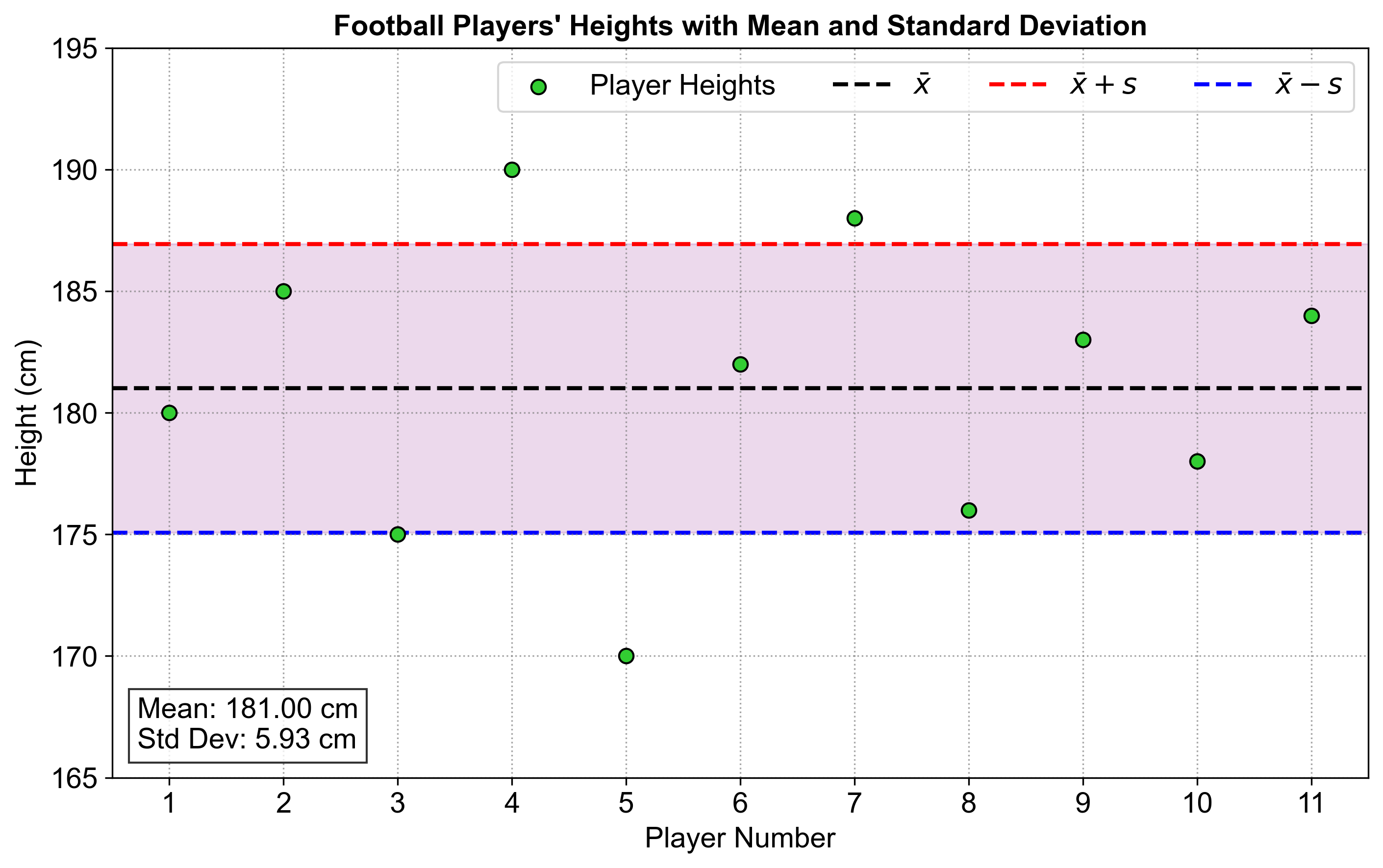
Figure Fig. 2.64 illustrates the individual heights of a group of football players (in centimeters) alongside their mean height and standard deviation:

• Data Points (Green Circles): Each green circle represents the height of an individual football player, numbered from 1 to 11 on the x-axis.

• Mean Height (Black Dashed Line): The black dashed line represents the average height of all players, denoted by \(\bar{x}\). This line indicates the central tendency of the data.

• Standard Deviation Range (Purple Shaded Area): The shaded purple area around the mean height shows one standard deviation above and below the mean, indicating the spread of most data points around the mean. It highlights the typical variability in player heights.

• Upper and Lower Standard Deviation Lines (Red and Blue Dashed Lines): The red dashed line represents \(\bar{x} + s\) (mean plus one standard deviation), and the blue dashed line represents \(\bar{x} - s\) (mean minus one standard deviation). These lines help in visualizing the range within which most player heights fall.

• Text Annotation: The lower-left corner includes a text box showing the mean and standard deviation values, providing a quick summary of the data’s central tendency and spread.

Fig. 2.64 Heights of Football Players with Mean and Standard Deviation.

Note

The following equations

(2.29)\[s^2 = \dfrac{1}{n-1}\left( \sum_{i=1}^{n} x_i^2 - n\bar{x}^2\right)\]

or

(2.30)\[s^2 = \frac{1}{n - 1} \left( \sum_{i=1}^{n} x_i^2 - \frac{1}{n} \left(\sum_{i=1}^{n} x_i \right)^2 \right)\]

are simplifications of the formula for calculating the sample variance. It’s a way to compute the variance more efficiently, especially when dealing with large datasets.

How we get from equation (2.29) to equation (2.30)?

Note that, We start with the definition of sample variance:

\[\begin{equation*}s^2 = \frac{1}{n - 1}\sum_{i=1}^{n} (x_i - \bar{x})^2\end{equation*}\]

This formula tells us to subtract the sample mean \( \bar{x} \) from each data point \( x_i \), square the result, and then sum all those squared differences. Finally, we divide by \( n - 1 \) to get the sample variance.

Now, let’s expand the squared term inside the summation:

\[\begin{equation*}(x_i - \bar{x})^2 = x_i^2 - 2x_i\bar{x} + \bar{x}^2\end{equation*}\]

When we sum over all data points, we get:

\[\begin{equation*}\sum_{i=1}^{n} (x_i - \bar{x})^2 = \sum_{i=1}^{n} x_i^2 - 2\bar{x}\sum_{i=1}^{n} x_i + n\bar{x}^2\end{equation*}\]

But since \( \bar{x} \) is the average of all \( x_i \)‘s, we know that:

\[\begin{equation*}\sum_{i=1}^{n} x_i = n\bar{x}\end{equation*}\]

Substituting this into our expanded summation gives us:

\[\begin{equation*}\sum_{i=1}^{n} (x_i - \bar{x})^2 = \sum_{i=1}^{n} x_i^2 - 2n\bar{x}^2 + n\bar{x}^2\end{equation*}\]

\[\begin{equation*}\sum_{i=1}^{n} (x_i - \bar{x})^2 = \sum_{i=1}^{n} x_i^2 - n\bar{x}^2\end{equation*}\]

Now, we can substitute \(n\bar{x}^2\) with \((\sum_{i=1}^{n} x_i)^2 / n\) because \(n\bar{x}^2\) is just the square of the sum of all \(x_i\)’s divided by \(n\) (since \(\bar{x} = \sum_{i=1}^{n} x_i / n\)):

\[\begin{equation*}\sum_{i=1}^{n} (x_i - \bar{x})^2 = \sum_{i=1}^{n} x_i^2 - \frac{1}{n}\left(\sum_{i=1}^{n} x_i \right)^2\end{equation*}\]

Finally, we substitute this back into the original variance formula:

\[\begin{equation*}s^2 = \frac{1}{n - 1} \left( \sum_{i=1}^{n} x_i^2 - \frac{1}{n} \left(\sum_{i=1}^{n} x_i \right)^2 \right).\end{equation*}\]

Computing Formula for a Sample Standard Deviation

The sample standard deviation (s) is a statistical measure that quantifies the dispersion or spread of data within a sample. It provides an estimate of how much individual data points deviate from the sample mean.

1. Sample Standard Deviation (s):

   • The sample standard deviation is denoted by s.

   • It measures the variability or dispersion of data points in a sample.

2. Formula for Sample Standard Deviation:

   • The formula to calculate the sample standard deviation is as follows:

     (2.31)\[\begin{equation} s = \sqrt{\frac{1}{n - 1} \left( \sum_{i=1}^{n} x_i^2 - \frac{1}{n} \left(\sum_{i=1}^{n} x_i \right)^2 \right)} \end{equation}\]

3. Components of the Formula:

   • \(n\) represents the sample size (number of data points).

   • \(\sum x\) denotes the sum of all individual data points in the sample.

   • \(\sum x^2\) represents the sum of the squares of each data point in the sample.

4. Step-by-Step Calculation:

   • Calculate the sum of the data points: \(\sum x\).

   • Compute the sum of the squares of each data point: \(\sum x^2\).

   • Subtract the square of the sum of data points from the sum of squares: \(\dfrac{(\sum x)^2}{n}\).

   • Divide this result by \((n-1)\).

   • Finally, take the square root of the entire expression to obtain the sample standard deviation \(s\).

5. Purpose:

   • The sample standard deviation helps estimate the population standard deviation based on the available sample data.

   • It provides an unbiased estimate of the variability in the entire population.

2.8.3. Population Variance and Standard Deviation

The population variance, denoted as \(\sigma^2\), quantifies the spread or variability of data points within an entire population. It provides insights into how individual data points deviate from the population mean. The formula for population variance is:

(2.32)\[\begin{equation} \sigma^2 = \dfrac{1}{N} \sum_{i=1}^{N}{(x_{i} - \mu)^2} \end{equation}\]

Where:

• \(x\) represents individual data points from the population.

• \(\mu\) denotes the population mean (average).

• \(\sum\) signifies the sum of squared deviations from the mean.

• \(N\) is the total number of data points in the population.

The population standard deviation, denoted by the Greek letter \(\sigma\) (sigma), is used when considering an entire population. It provides insights into how much individual data points deviate from the population mean. Here’s how we calculate it:

1. Formula for Population Standard Deviation:

   • The population standard deviation is calculated using the following formula:

     (2.33)\[\begin{equation} \sigma = \sqrt{\dfrac{1}{N} \sum_{i=1}^{N}{(x_{i} - \mu)^2} } \end{equation}\]

     where:

     • \(x\) represents individual data points from the population.

     • \(\mu\) denotes the population mean (average).

     • \(\sum\) signifies the sum of all the squared deviations from the mean.

     • \(N\) is the total number of data points in the population.

2. Step-by-Step Calculation:

   • Compute the deviation of each data point from the population mean: \(x - \mu\).

   • Square each deviation: \((x - \mu)^2\).

   • Sum up all the squared deviations: \(\sum_{i=1}^{N}{(x_{i} - \mu)^2}\).

   • Divide this sum by the population size \(N\).

   • Finally, take the square root of the entire expression to obtain the population standard deviation \(\sigma\).

3. Interpretation:

   • The population standard deviation provides a measure of how spread out the data points are within the entire population.

   • It is expressed in the original units of the data.

When working with statistical calculators, keep in mind that they often provide both the sample standard deviation (\(s\)) and the population standard deviation (\(\sigma\)). The latter is computed using the formula that directly divides by the population size \(N\). Different calculators may use varying notations to represent these two types of standard deviations.

2.8.4. Variance of a Sample and a Population

The variance of a set of values measures the variation or spread within that dataset. It corresponds to the square of the standard deviation. We encounter two types of variance:

1. Sample Variance:

   • Denoted as \(s^2\), it is the square of the sample standard deviation \(s\).

   • Sample variance quantifies how data points deviate from the sample mean.

   • Formula:

     (2.34)\[\begin{equation} s^2 = \dfrac{1}{n-1} \sum_{i=1}^{n}{(x_{i} - \bar{x})^2} \end{equation}\]

     where:

     • \(x\) represents individual data points from the sample.

     • \(\bar{x}\) denotes the sample mean (average).

     • \(\sum\) signifies the sum of squared deviations from the mean.

     • \(n\) is the sample size.

2. Population Variance:

   • Denoted as \(\sigma^2\), it is the square of the population standard deviation \(\sigma\).

   • Population variance provides insights into how data points deviate from the population mean.

   • Formula:

     (2.35)\[\begin{equation} \sigma^2 = \dfrac{1}{N} \sum_{i=1}^{N}{(x_{i} - \mu)^2}\end{equation}\]

     where:

     • \(x\) represents individual data points from the population.

     • \(\mu\) denotes the population mean.

     • \(\sum\) signifies the sum of squared deviations from the mean.

     • \(N\) is the total number of data points in the population.

Table 2.1 A summary of the notation for standard deviation and variance: Sample standard deviation (\(s\)), Sample variance (\(s^2\)), Population standard deviation (\(\sigma\)), and Population variance (\(\sigma^2\))

Measure	Formula
Sample Standard Deviation	\(\displaystyle{s = \sqrt{\dfrac{1}{n-1} \sum_{i=1}^{n}{(x_{i} - \bar{x})^2} }}\)
Sample Variance	\(\displaystyle{s^2 = \dfrac{1}{n-1} \sum_{i=1}^{n}{(x_{i} - \bar{x})^2}}\)
Population Standard Deviation	\(\displaystyle{\sigma = \sqrt{\dfrac{1}{N} \sum_{i=1}^{N}{(x_{i} - \mu)^2}}}\)
Population Variance	\(\displaystyle{\sigma^2 = \dfrac{1}{N} \sum_{i=1}^{N}{(x_{i} - \mu)^2}}\)

Example 2.55

A researcher is studying the consistency of a chemical solution’s concentration in a series of experiments. The following numbers represent the concentration measurements (in percentage) from 12 different trials:

Measurements: 27.0, 26.8, 27.1, 27.3, 27.4, 27.7, 28.1, 27.9, 28.3, 28.2, 28.3, 28.4

• a. Calculate the Range.

• b. Compute the Variance.

• c. Determine the Standard Deviation.

Solution:

a. Range: The range is the difference between the maximum value and the minimum value in the dataset.

• Maximum value: \(28.4\)

• Minimum value: \(26.8\)

\[\begin{align*}\text{Range} &= \text{Maximum value} - \text{Minimum value}\\ &= 28.4 \text{ Percent} − 26.8 \text{ Percent} = 1.6 \text{ Percent}\end{align*}\]

Fig. 2.65 Visualizing the Range for Example 2.55.

b. Variance: The variance measures the spread or variability of data points around the mean. For a sample, we use the sample variance formula:

\[\begin{equation*}s^2 = \dfrac{n\left(\sum x^2\right) - \left(\sum x\right)^2}{n(n-1)}\end{equation*}\]

Let’s calculate step by step:

1. Calculate \(\sum x\):

   \[\begin{equation*}\sum x = 332.5\end{equation*}\]

2. Calculate \(\sum x^2\):

   \[\begin{equation*}\sum x^2 = 9216.59\end{equation*}\]

3. Calculate \(n\left(\sum x^2\right)\):

   \[\begin{equation*}n\left(\sum x^2\right) = 12 \cdot 9216.59 = 110599.08\end{equation*}\]

4. Calculate \(\left(\sum x\right)^2\):

   \[\begin{equation*}\left(\sum x\right)^2 = (332.5)^2 = 110556.25\end{equation*}\]

5. Compute the sample variance:

   \[\begin{equation*}s^2 = \dfrac{110599.08 - 110556.25}{12 \cdot 11} = 0.324\end{equation*}\]

c. Standard Deviation: The standard deviation is the square root of the variance:

\[\begin{equation*}s = \sqrt{s^2} = \sqrt{0.324} = 0.57\end{equation*}\]

Therefore:

• Range = 1.6

• Sample Variance (\(s^2\)) = 0.324

• Sample Standard Deviation (\(s\)) = 0.57

Example 2.56

Measured amounts of caffeine (mg per 12 oz of drink) obtained from one can for each of 20 brands:

0, 0, 34, 34, 34, 45, 41, 51, 55, 36, 47, 41, 0, 0, 53, 54, 38, 0, 41, 47

Find the range, variance, and standard deviation for the given sample data.

Solution:

a. Range: The range is the difference between the maximum value and the minimum value in the dataset.

• Maximum value: \(55\)

• Minimum value: \(0\)

\[\begin{align*}\text{Range} &= \text{Maximum value} - \text{Minimum value}\\ &= 55 - 0 = 55\text{ mg per 12 oz of drink}\end{align*}\]

Fig. 2.66 Visualizing the Range for Example 2.56.

b. Variance: The variance measures the spread or variability of data points around the mean. For a sample, we use the sample variance formula:

\[\begin{equation*}s^2 = \dfrac{n\left(\sum x^2\right) - \left(\sum x\right)^2}{n(n-1)}\end{equation*}\]

Let’s calculate step by step:

1. Calculate \(\sum x\):

   \[\begin{equation*}\sum x = 651\end{equation*}\]

2. Calculate \(\sum x^2\):

   \[\begin{equation*}\sum x^2 = 29045\end{equation*}\]

3. Calculate \(n\left(\sum x^2\right)\):

   \[\begin{equation*}n\left(\sum x^2\right) = 20 \cdot 29045 = 580900\end{equation*}\]

4. Calculate \(\left(\sum x\right)^2\):

   \[\begin{equation*}\left(\sum x\right)^2 = (651)^2 = 424401\end{equation*}\]

5. Compute the sample variance:

   \[\begin{equation*}s^2 = \dfrac{580900 - 424401}{20 \cdot 19} = 413.418\end{equation*}\]

c. Standard Deviation:

The standard deviation is the square root of the variance:

\[\begin{equation*}s = \sqrt{s^2} = \sqrt{413.418} = 20.333\end{equation*}\]

Therefore:

• Range = 55

• Sample Variance (\(s^2\)) = 413.4

• Sample Standard Deviation (\(s\)) = 20.3

Example 2.57

Imagine you are a botanist studying a rare species of plant found in the Amazon rainforest. These plants are known for their rapid growth and unique flowering patterns. You’ve measured the heights of 10 randomly selected plants (in millimeters) during the peak growth season to understand their growth distribution. The data you’ve collected is as follows:

Given Data (heights in millimeters):

37.5, 31.5, 27.4, 21, 32, 33, 33, 38, 17.4, 34.5

Analyze the data to determine the mean, median, mode, range, and standard deviation. This will help you understand the average height, the variability, and the most common height among these plants.

Solution:

a. Mean (Average Height): The mean height is calculated by adding all the heights together and dividing by the number of plants:

\[\begin{equation*}\text{Mean} = \dfrac{\sum \text{heights}}{\text{number of plants}} = \dfrac{37.5 + 31.5 + 27.4 + 21 + 32 + 33 + 33 + 38 + 17.4 + 34.5}{10}\end{equation*}\]

b. Median: Since the sample size (\(n\)) is even (10), we find the median by taking the mean of the two middle observations in the ordered list of data values:

\[\begin{equation*}\text{Ordered data:} \quad 17.4, 21.0, 27.4, 31.5, 32.0, 33.0, 33.0, 34.5, 37.5, 38.0\end{equation*}\]

\[\begin{equation*}\text{Median} = \dfrac{32 + 33}{2} = 32.5\end{equation*}\]

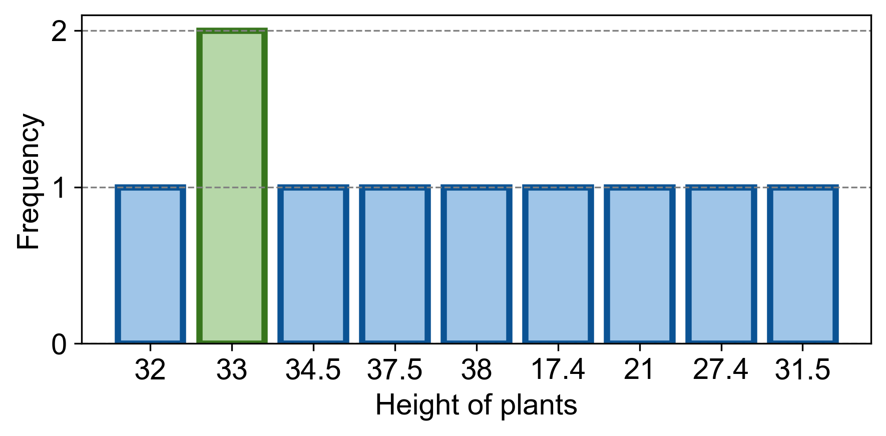
c. Mode: The mode is the most frequently occurring value. Since \(33.0\) occurs twice and no other value occurs more than once, the mode is \(33.0\).

Fig. 2.67 Visualizing the Mode for Example 2.57.

d. Range: The range is the difference between the maximum and minimum values:

\[\begin{equation*}\text{Range} = \text{Maximum} - \text{Minimum} = 38 - 17.4 = 20.6\end{equation*}\]

Fig. 2.68 Visualizing the Range for Example 2.57.

e. Standard Deviation: The sample standard deviation (\(s\)) can be calculated using two equivalent formulas:

1. Using the definition formula:

\[\begin{equation*} s = \sqrt{\frac{\sum_{i=1}^{n} (x_i - \overline{x})^2}{n - 1}} \end{equation*}\]

2. Using the computational formula:

\[\begin{equation*} s = \sqrt{\frac{n\sum x_i^2 - (\sum x_i)^2}{n(n-1)}} \end{equation*}\]

Let’s calculate using both methods:

Method 1: Definition Formula

Step 1: Calculate the mean (\(\overline{x}\))

\[\begin{equation*} \overline{x} = \frac{\sum_{i=1}^{n} x_i}{n} = \frac{305.30}{10} = 30.53 \end{equation*}\]

Step 2: Calculate \((x_i - \overline{x})^2\) for each data point

\(x_i\)	\(x_i - \overline{x}\)	\((x_i - \overline{x})^2\)
37.5	6.97	48.5809
31.5	0.97	0.9409
27.4	-3.13	9.7969
21.0	-9.53	90.8209
32.0	1.47	2.1609
33.0	2.47	6.1009
33.0	2.47	6.1009
38.0	7.47	55.8009
17.4	-13.13	172.3970
34.5	3.97	15.7609

Step 3: Sum the \((x_i - \overline{x})^2\) values

\[\begin{equation*} \sum_{i=1}^{n} (x_i - \overline{x})^2 = 408.4611 \end{equation*}\]

Step 4: Apply the formula

\[\begin{equation*} s = \sqrt{\frac{408.4611}{10 - 1}} = \sqrt{45.3846} \approx 6.737 \end{equation*}\]

Method 2: Computational Formula

Given:

• \(n = 10\)

• \(\sum x_i = 305.30\)

• \(\sum x_i^2 = 9729.27\)

Step 1: Calculate \(n\sum x_i^2\)

\[\begin{equation*} n\sum x_i^2 = 10 \times 9729.27 = 97292.70 \end{equation*}\]

Step 2: Calculate \((\sum x_i)^2\)

\[\begin{equation*} (\sum x_i)^2 = 305.30^2 = 93208.09 \end{equation*}\]

Step 3: Apply the formula

\[\begin{equation*} s = \sqrt{\frac{97292.70 - 93208.09}{10(10-1)}} = \sqrt{\frac{4084.61}{90}} = \sqrt{45.3846} \approx 6.737 \end{equation*}\]

Therefore, using both methods, we confirm that the sample standard deviation (\(s\)) is approximately 6.737 mm.

Interpretation: The standard deviation of 6.737 mm indicates that, on average, the plant heights in this sample deviate from the mean height by about 6.737 mm. This measure provides insight into the variability of plant heights in the studied population.