4.3. Binomial Distribution#
4.3.1. Binomial Coefficients: An Introduction#
Let’s start with a simple example to understand the concept of binomial coefficients. Imagine we have three students: Alice, Bob, and Charlie. We want to know how many ways we can choose 2 students from this group of 3.
Let’s list out all the possible combinations:
Alice and Bob
Alice and Charlie
Bob and Charlie
We can see that there are 3 different ways to choose 2 students from a group of 3.
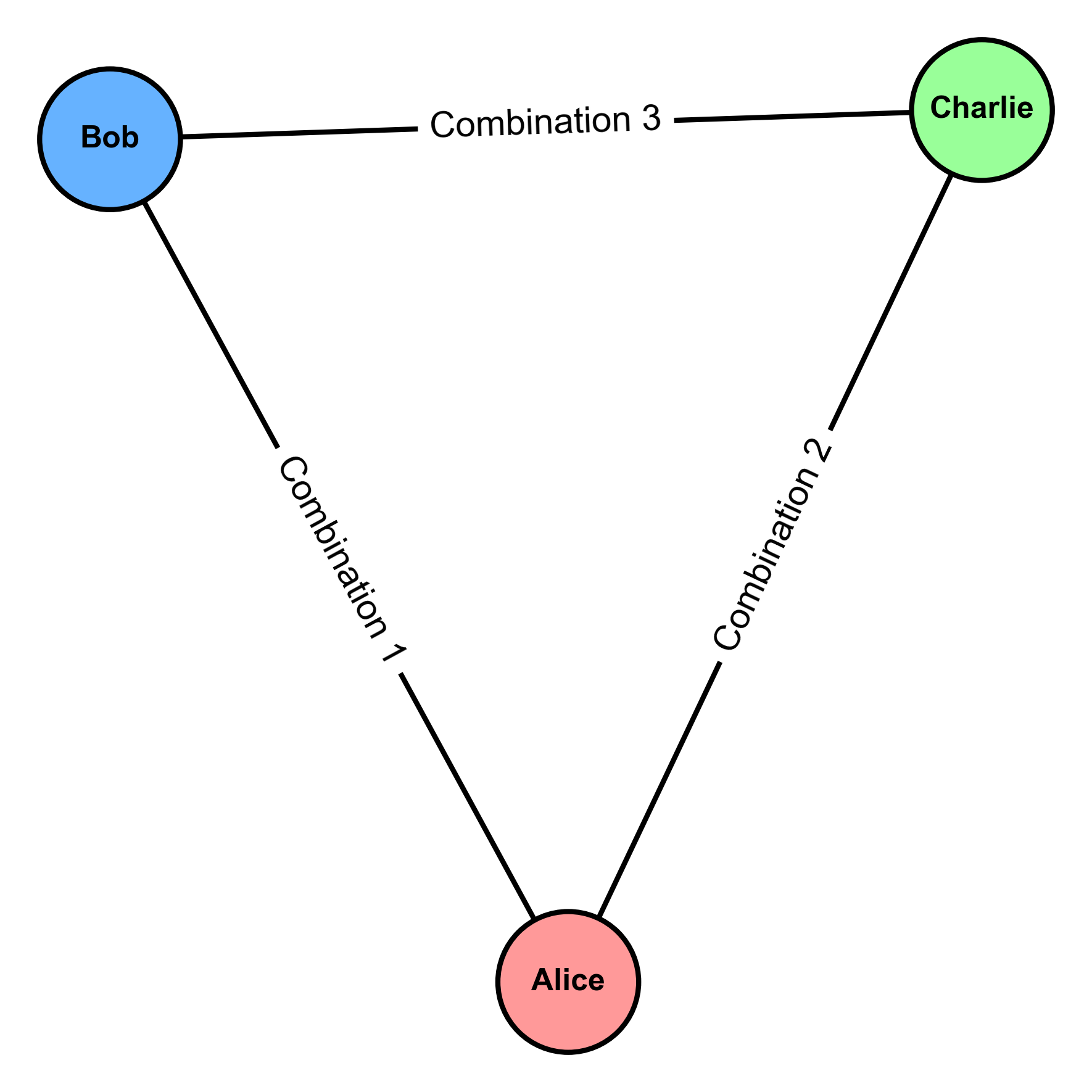
Fig. 4.12 Visual representation of the three possible combinations when choosing 2 students from a group of 3. Each node represents a student, and each connecting line represents a combination. The labels on the lines indicate the specific combinations.#
This approach of listing all possibilities works well for small sets. However, imagine if we needed to choose 2 students from a class of 20. Listing all combinations would be time-consuming and prone to errors. We need a mathematical way to calculate this quickly and accurately.
This is where the concept of binomial coefficients comes in. To understand binomial coefficients, we first need to introduce the concept of factorials.
4.3.2. Factorials#
The factorial of a non-negative integer \(k\), denoted by \(k!\), is the product of all positive integers less than or equal to \(k\). Formally, it’s defined as:
For the base case, we define \(0!\) as \(1\) to make the definition coherent for mathematical operations involving factorials, such as the calculation of permutations and combinations.
Example 4.16 (Factorial)
Calculate \( 5! \).
Solution:
So, \(5!\) equals \(120\).
Using factorials, we can define the binomial coefficient, which gives us a formula to calculate the number of ways to choose \(k\) items from a set of \(n\) items, regardless of order.
4.3.3. Binomial Coefficients#
The binomial coefficient is a mathematical construct that quantifies the number of possible combinations of \(k\) elements from a set of \(n\) distinct elements. Represented by \(\binom{n}{k}\), it is a crucial component in both algebraic and statistical contexts.
In algebra, the binomial coefficient is central to the binomial theorem, which describes the expansion of \((a + b)^n\). It dictates the coefficients of the terms in this expansion. Mathematically, the binomial coefficient is defined as:
where \(n!\) denotes the factorial of \(n\), the product of all positive integers up to \(n\).
From a combinatorial perspective, the binomial coefficient reflects the concept of combinations, where the order of selection does not matter. This is different from permutations, where the order is significant.
In statistics, binomial coefficients are integral to binomial distributions, which model scenarios with a fixed number of independent trials, each with the same probability of success. They help calculate the probabilities of observing various numbers of successes.
Example 4.17 (Binomial Coefficient)
Find the binomial coefficient \(\displaystyle{\binom{5}{2}}\).
Solution:
Thus, \(\binom{5}{2}\) is \(10\), which means there are 10 different ways to choose 2 items from a set of 5.
Example 4.18 (Application in Probability)
Suppose you have a bowl with 6 different fruits, and you want to know how many ways you can pick 3 fruits.

Fig. 4.13 A bowl with 6 different fruits. Image generated by Microsoft Designer.#
Solution: We can use the binomial coefficient to solve this:
There are 20 different ways to pick 3 fruits from a set of 6.
These examples should help clarify how factorials and binomial coefficients work and how they can be applied in various mathematical contexts.
4.3.4. Characteristics of a Binomial Experiment#
Fixed Number of Trials (\(n\)): The total number of true-false questions Joe answers is the fixed number of trials in this experiment. Each question represents one trial.
Two Possible Outcomes: For each question (trial), there are only two possible outcomes: a “success” if Joe guesses correctly, or a “failure” if he guesses incorrectly.
Probability of Success (\(p\)) and Probability of Failure (\(q\)): Joe has a probability of success (\(p\)) of 0.6 for correctly guessing any given question. Conversely, the probability of failure (\(q\)), which is the chance of an incorrect guess, is 0.4. These probabilities are complementary, meaning \(p + q = 1\), which is a fundamental property of binomial experiments.
Independent Trials: The trials are independent; the result of one question does not influence the result of another. This independence ensures that Joe’s probabilities of success (\(p = 0.6\)) and failure (\(q = 0.4\)) are consistent across all trials.
This framework allows us to model and analyze the probability of various outcomes, such as the likelihood of Joe guessing a certain number of questions correctly, using binomial probability formulas.
Definition - Bernoulli Trials
A Bernoulli trial is a random experiment where:
Two Possible Outcomes: Each trial has exactly two mutually exclusive outcomes, typically labeled as “success” (s) and “failure” (f). Only one outcome can occur in each trial.
Independent Trials: The trials are independent, meaning the outcome of one trial does not affect the outcome of another. Each trial is an isolated event.
Constant Probability of Success: The probability of success, denoted by \(p\), remains constant across all trials. The probability of failure, denoted by \(q\), is \( 1 - p \), ensuring that \(p + q = 1\).
Bernoulli trials are foundational in probability theory and are used to model situations where there are two possible outcomes, such as flipping a coin or making a yes/no decision.
4.3.5. Understanding Bernoulli Trial#
In a sequence of \(n\) Bernoulli trials, each with two possible outcomes—success or failure—and where each trial is independent and has a constant probability of success \(p\), the binomial coefficient \(\binom{n}{x}\) quantifies the number of distinct outcomes with exactly \(x\) successes.
The binomial coefficient is computed as:
Here’s what each term represents:
\(n!\) (n factorial) is the product of all positive integers up to \(n\).
\( x! \) (x factorial) is the product of all positive integers up to \(x\).
\( (n-x)! \) is the factorial of the difference between \(n\) and \(x\).
The binomial coefficient, \(\binom{n}{x}\), thus denotes the number of ways to select \(x\) successes out of \(n\) trials, disregarding the sequence of these successes. This coefficient is pivotal in calculating probabilities in binomial distributions, which model scenarios like the one described.
Binomial Probability Formula
The binomial probability formula calculates the likelihood of observing a specific number of successes in a sequence of Bernoulli trials. Let’s denote \(x\) as the total number of successes in \(n\) trials, with the probability of success in each trial being \(p\). The probability that \(x\) equals a particular value \(x\) is given by:
Here, \(x\) is a binomial random variable and follows the binomial distribution with parameters \(n\) (number of trials) and \(p\) (probability of success).
Example 4.19
Find the probability of achieving exactly 3 successes in 5 Bernoulli trials, where the probability of success is \(p\), use the binomial coefficient:
Solution:
In this formula:
\(p^{3}\) signifies the probability of achieving 3 successes.
\((1 - p)^{2}\) signifies the probability of experiencing 2 failures since failures are the complement of successes.
This formula is a powerful tool in statistics for modeling scenarios where outcomes are binary and each trial is independent.
Remark
For simplicity, the probability of failure can be shown with \(q\) where \(q = 1-p\).
4.3.6. Finding Binomial Probabilities#
The probability of observing exactly \(x\) successes in \(n\) trials is calculated using the binomial probability formula:
This formula combines the binomial coefficient (the number of ways to arrange \(x\) successes among \(n\) trials) with the probabilities of successes and failures raised to the appropriate powers.
Notation for the Binomial Distribution:**
\(B\): Binomial Probability Distribution Function
\(X \sim B(n, p)\): This denotes that \(x\) is a binomial random variable with \(n\) trials and a success probability \(p\) on each trial.
Using this notation and formulas, we can model and analyze scenarios where outcomes follow a binomial distribution.
Example 4.20 (Random Guesses in Multiple-Choice Questions)
Assume that random guesses are made for ten multiple-choice questions on an exam so that there are \(n = 10\) trials, each with a probability of success (correct) given by \(p = 0.25\). Find the indicated probability for the number of correct answers:
a. Find the probability that the number \(x\) of correct answers is exactly 8.
b. Find the probability that the number \(x\) of correct answers is at least 5.
c. Find the probability that the number \(x\) of correct answers is fewer than 4.
Solution: The binomial probability formula is given by:
Where:
\(n\) is the number of trials
\(k\) is the number of successful outcomes
\(p\) is the probability of success on a single trial
\(\binom{n}{k}\) is the binomial coefficient, calculated as \(\dfrac{n!}{k!(n-k)!}\)
For the exercise with \(n = 10\) trials and \(p = 0.25\) probability of success, we can calculate the probabilities as follows:
a. Exactly 8 correct answers (\(k = 8\)):
b. At least 5 correct answers (\(k \geq 5\)):
c. Fewer than 4 correct answers (\(k < 4\)):
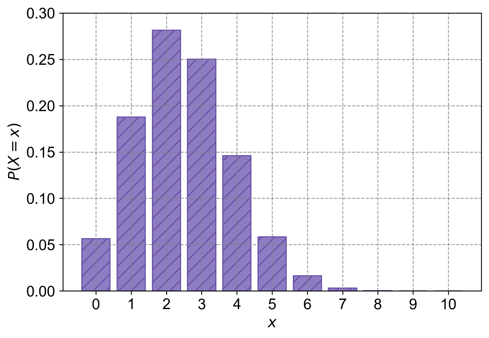
Fig. 4.14 The probability mass function (PMF) for a binomial distribution with \(n = 10\) trials and \(p = 0.25\). The random variable \(X\) represents the number of correct answers in a multiple-choice exam with random guessing for each question. Each bar shows the probability of observing exactly \(x\) correct answers, where \(x\) ranges from 0 to 10.#
Example 4.21 (Random Guesses in Multiple-Choice Questions)
Assume that random guesses are made for twelve multiple-choice questions on an exam so that there are \(n = 12\) trials, each with a probability of success (correct) given by \(p = 1/6\). Find the indicated probability for the number of correct answers:
a. Find the probability that the number \(x\) of correct answers is exactly 9.
b. Find the probability that the number \(x\) of correct answers is at least 6.
c. Find the probability that the number \(x\) of correct answers is fewer than 4.
Solution:
The binomial probability formula is given by:
Where:
\(n\) is the number of trials
\(k\) is the number of successful outcomes
\(p\) is the probability of success on a single trial
\(\binom{n}{k}\) is the binomial coefficient, calculated as \(\dfrac{n!}{k!(n-k)!}\)
For this exercise with \(n = 12\) trials and \(p = \frac{1}{6}\) probability of success, we calculate:
a. Exactly 9 correct answers (\(k = 9\)):
b. At least 6 correct answers (\(k \geq 6\)):
c. Fewer than 4 correct answers (\(k < 4\)):
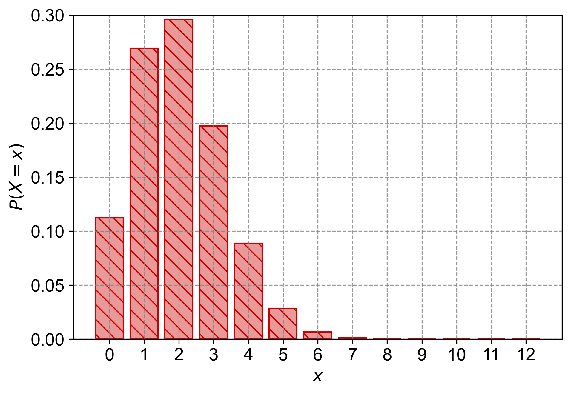
Fig. 4.15 The probability mass function (PMF) for a binomial distribution with \(n = 12\) trials and \(p = \frac{1}{6}\). The random variable \(X\) represents the number of correct answers in a multiple-choice exam with random guessing for each question. Each bar shows the probability of observing exactly \(x\) correct answers, where \(x\) ranges from 0 to 12.#
4.3.7. Mean and Standard Deviation of a Binomial Random Variable#
For a binomial random variable \(x\) with parameters \(n\) (number of trials) and \(p\) (probability of success), the mean (expected value) and standard deviation are given by:
Mean (\(\mu\)): The average number of successes expected.
The mean depends on both the number of trials (\(n\)) and the probability of success (\(p\)). The following figure illustrates how the mean changes as a function of \(p\) for different values of \(n\):
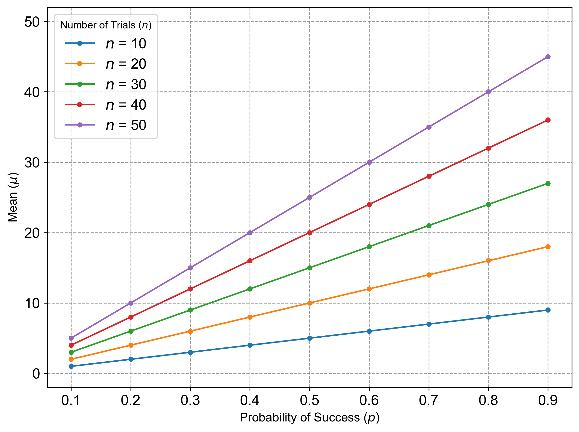
Fig. 4.16 The mean (\(\mu = np\)) of a binomial random variable as a function of the probability of success (\(p\)) for different numbers of trials (\(n\)). As \(p\) increases, the mean increases linearly for a fixed \(n\).#
Variance (\(\sigma^2\)): The measure of the spread of the distribution.
Standard Deviation (\(\sigma\)): The square root of the variance, indicating the typical distance of the data from the mean.
The standard deviation depends on both \(n\) and \(p\), but unlike the mean, it is not linear in \(p\). The following figure shows how the standard deviation changes as a function of \(p\) for different values of \(n\):
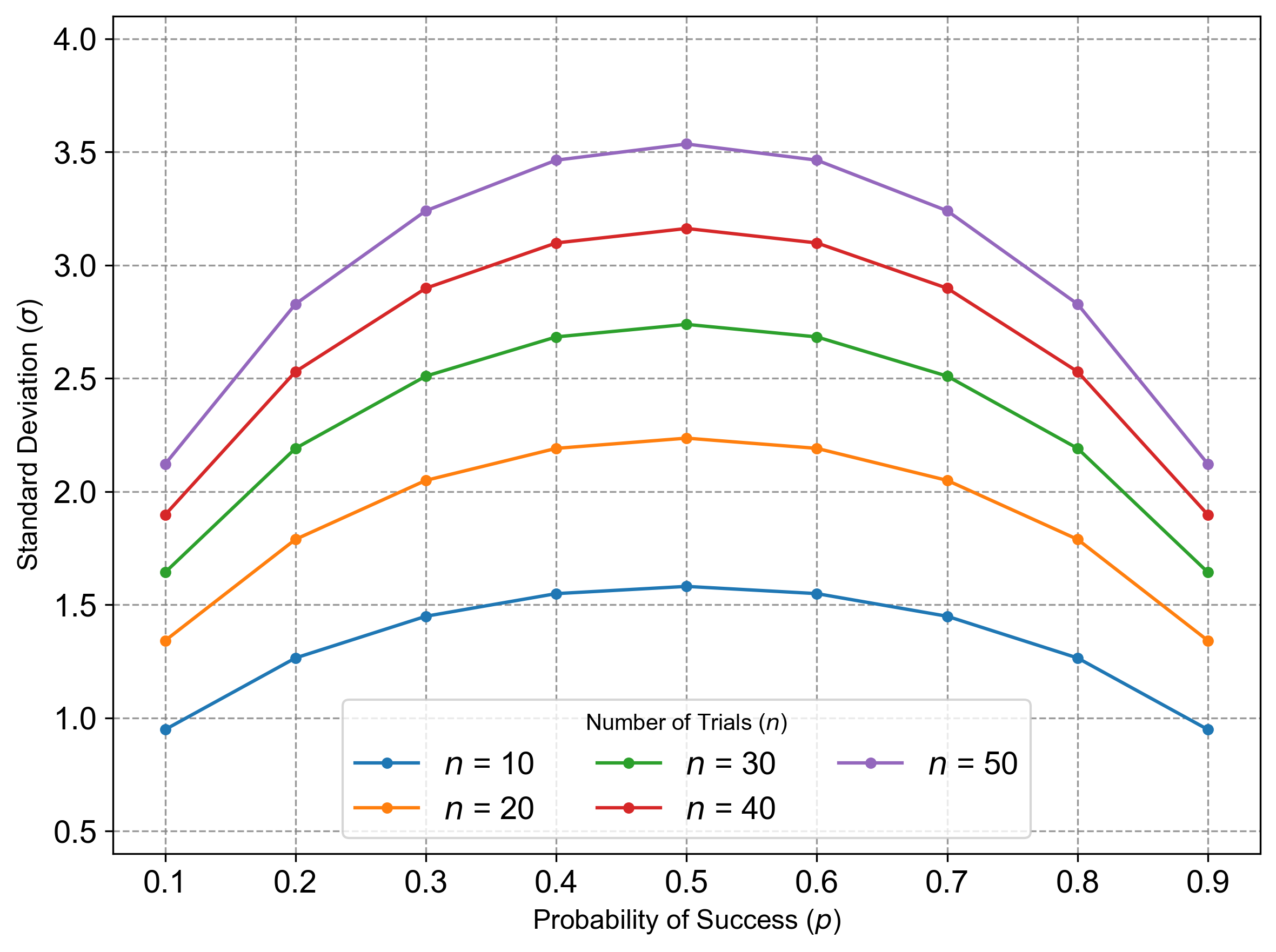
Fig. 4.17 The standard deviation (\(\sigma = \sqrt{np(1-p)}\)) of a binomial random variable as a function of the probability of success (\(p\)) for different numbers of trials (\(n\)). The standard deviation is maximized at \(p = 0.5\), reflecting the greatest uncertainty in outcomes.#
Observations:
Mean (\(\mu = np\)):
The mean increases linearly with \(p\), as shown in the first figure.
For a fixed number of trials (\(n\)), higher probabilities result in higher expected values.
Standard Deviation (\(\sigma = \sqrt{np(1-p)}\)):
The standard deviation is maximized when \(p = 0.5\), as this is where variability is greatest.
For very small or very large values of \(p\), the standard deviation decreases, reflecting lower uncertainty in outcomes.
Example 4.22
According to a health report, the rate of natural birth (without C-section) in a certain region is approximately p = 40%. Suppose we select a random sample of deliveries from a hospital. Of the n = 20 delivery records pulled for a particular year:
a. What is the probability that at most 5 babies were delivered without C-section?
b. What is the probability that more than 5 babies were delivered without C-section?
c. What is the mean (expected value) and standard deviation of the number of babies delivered without C-section?
Solution: Given:
The probability of natural birth \(p = 0.40\)
The number of delivery records \(n = 20\)
We can calculate the following:
a. The probability that at most 5 babies were delivered without C-section is given by the cumulative distribution function:
b. The probability that more than 5 babies were delivered without C-section is the complement of the CDF for \(k \leq 5\):
c. The mean (expected value) \(\mu\) and standard deviation \(\sigma\) for the binomial distribution are given by:
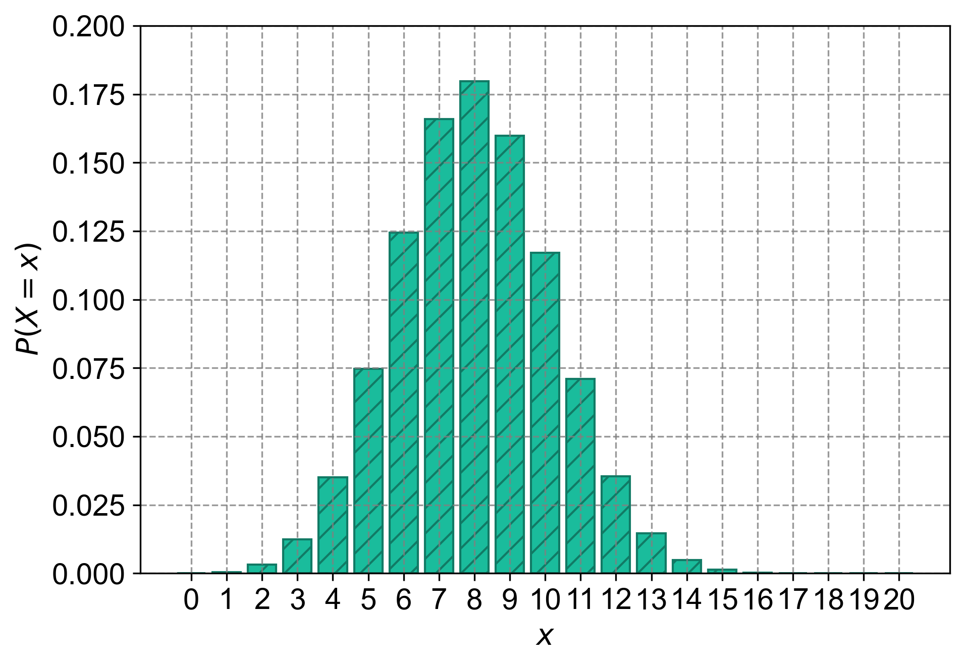
Fig. 4.18 The probability mass function (PMF) for a binomial distribution with \(n = 20\) trials and \(p = 0.40\). Each bar represents the probability of observing exactly \(x\) successes, where \(x\) ranges from \(0\) to \(20\). The y-axis shows the corresponding probabilities.#
Example 4.23
Let \(X\) be a binomial random variable with the mean \(\mu = 6\) and variance \(\sigma^2 = 2.4\). Find
a. \(P(X = 3)\)
b. \(P(X > 14)\).
Solution: First, we need to determine the number of trials \(n\) and the probability of success \(p\) using the given mean and variance.
For a binomial distribution:
Given: \(\mu = 6\) and \(\sigma^2 = 2.4\)
From these, we can set up two equations:
Dividing the second equation by the first:
Now that we know \(p\), we can solve for \(n\) using the mean equation:
Thus, we’ve derived that \(n = 10\) and \(p = 0.6\).
Now we can calculate the probabilities:
a) \(P(X = 3)\):
b) \(P(X > 14)\): Since \(n = 10\), it’s impossible for \(X\) to be greater than 14. Therefore:
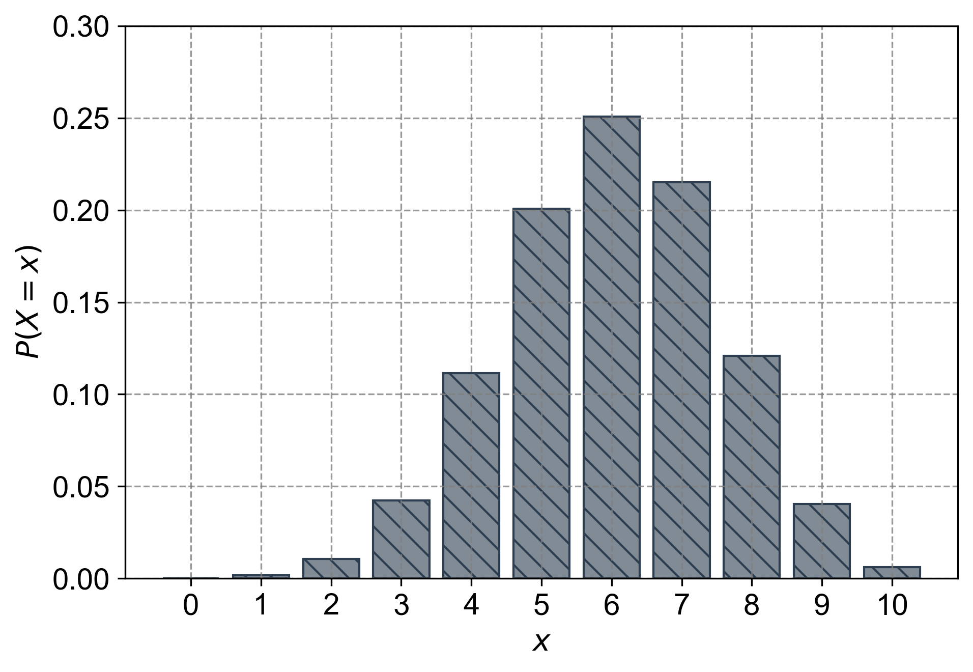
Fig. 4.19 The probability mass function (PMF) for a binomial distribution with \(n = 10\) trials and \(p = 0.60\). Each bar represents the probability of observing exactly \(x\) successes, where \(x\) ranges from \(0\) to \(10\). The y-axis shows the corresponding probabilities.#
Example 4.24
A consumer survey suggests that around 10% of smartphones have a specific software issue that has not been fixed with an update. A technician checks 15 smartphones at random. What is the probability that fewer than five of them have this software issue?
Solution: Let \(Y\) represent the number of smartphones in the sample that have the software issue but have not been updated. Then \(Y\) follows a binomial distribution with parameters \(n = 15\) and \(p = 0.1\). The probability that fewer than five have the software issue is \(P(Y < 5)\).
To solve this, we sum the probabilities of \(Y\) being 0, 1, 2, 3, and 4:
Using the binomial probability formula:
We calculate each term:
Adding these up gives us:
Therefore, the probability that fewer than five out of 15 randomly checked smartphones have the software issue is approximately 0.987280 or 98.73%.
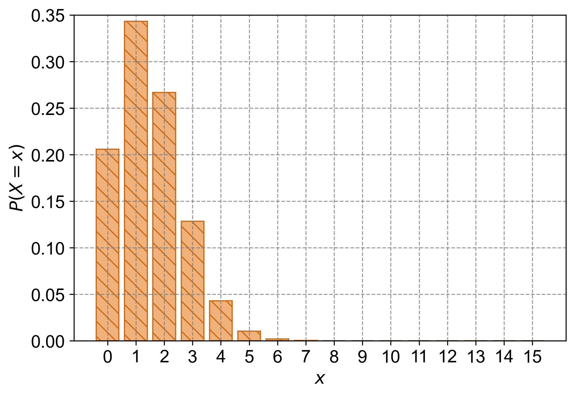
Fig. 4.20 The probability mass function (PMF) for a binomial distribution with \(n = 15\) trials and \(p = 0.10\). Each bar represents the probability of observing exactly \(y\) smartphones with the software issue, where \(y\) ranges from \(0\) to \(15\). The y-axis shows the corresponding probabilities.#
Example 4.25
In a small town, it is estimated that 30% of households own a dog. A local veterinarian selects 10 households at random for a study. What is the probability that at most three of the selected households own a dog?
Solution: Let \(D\) represent the number of households that own a dog. Then \(D\) follows a binomial distribution with parameters \(n=10\) and \(p=0.3\). The probability that at most three households own a dog is \(P(D \leq 3)\).
To solve this, we can sum the probabilities of \(D\) being 0, 1, 2, and 3:
Using the binomial probability formula:
We calculate each term:
Adding these up gives us \(P(D \leq 3)\):
So, there’s approximately a 64.96% chance that at most three out of the 10 randomly selected households will own a dog.
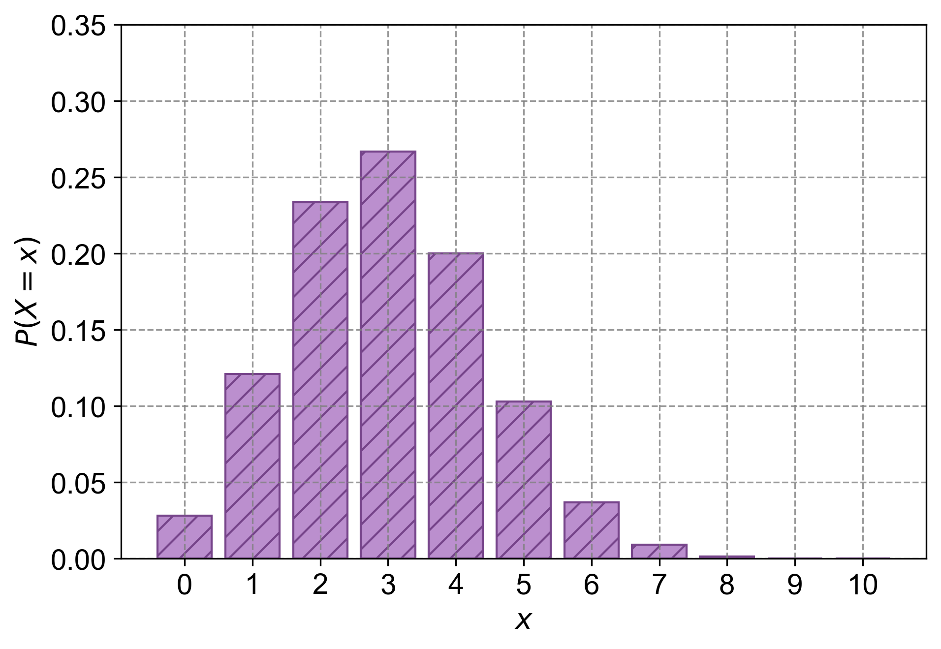
Fig. 4.21 The probability mass function (PMF) for a binomial distribution with \(n = 10\) trials and \(p = 0.30\). Each bar represents the probability of observing exactly \(d\) households owning a dog, where \(d\) ranges from \(0\) to \(10\). The y-axis shows the corresponding probabilities.#
4.3.8. Estimating Success Probability with Sample Proportion#
When dealing with Bernoulli trials, the true success probability, denoted as \(p\), is often unknown. To estimate \(p\), we can perform \(n\) independent trials and tally the number of successes, \(x\). The sample proportion, represented as \( \hat{p} \), serves as our estimate for \(p\):
This notation is part of a standard convention where the actual success probability is \(p\), and the sample proportion is \( \hat{p} \). The “hat” symbol over \(p\) signifies that \( \hat{p} \) is an estimator for the unknown parameter \(p\).
Example 4.26
A bakery manager is monitoring the weight consistency of loaves of bread. In a sample of 25 loaves, 5 are found to be lighter than the specified weight. Estimate the probability \(p\) that a loaf of bread is lighter than the specified weight.
Solution: The sample proportion of loaves that are lighter than the specified weight is calculated as the number of lighter loaves divided by the total number of loaves sampled. Therefore, the sample proportion \( \hat{p} \) is:
We estimate that the probability that a loaf of bread is lighter than the specified weight is 0.20.
