7.4. One-Tail, Two-Tail Tests, and Critical Values#
Hypothesis tests can be categorized into one-tail and two-tail tests based on the direction of the alternative hypothesis.
7.4.1. One-Tail Tests#
A one-tail test examines whether the sample data significantly deviate from the null hypothesis in one specific direction. It is used when the research hypothesis predicts a particular direction of the effect.
Left-Tailed Test:
The alternative hypothesis states that the population parameter is less than the null hypothesis value.
Example: \(H_a: \mu < \mu_0\)
Used when the research question is interested in finding evidence that the population mean is less than a specific value.
Right-Tailed Test:
The alternative hypothesis states that the population parameter is greater than the null hypothesis value.
Example: \(H_a: \mu > \mu_0\)
Used when the research question is interested in finding evidence that the population mean is greater than a specific value.
7.4.2. Two-Tail Test#
A two-tail test examines whether the sample data significantly deviate from the null hypothesis in either direction. It is used when the research hypothesis does not predict the direction of the effect, only that there will be a difference.
The alternative hypothesis states that the population parameter is different from the null hypothesis value.
Example: \(H_a: \mu \neq \mu_0\)
Used when the research question is interested in finding evidence that the population mean is different from a specific value, regardless of whether it is higher or lower.
Choosing Between One-Tail and Two-Tail Tests
The choice between a one-tail and a two-tail test depends on the research question and hypothesis. A one-tail test is more powerful in detecting an effect in the specified direction but cannot detect an effect in the opposite direction. A two-tail test is more conservative and can detect deviations in both directions but requires a larger effect size to reach statistical significance.
7.4.3. Test Statistic#
Before we discuss rejection regions and critical values, it’s essential to understand what a test statistic is in the context of hypothesis testing.
Definition - Test Statistic
A test statistic is a numerical value calculated from sample data that is used to decide whether to reject the null hypothesis. It quantifies how closely the sample data align with the null hypothesis.
The test statistic serves as a standardized measure that allows us to compare our sample results to what we would expect if the null hypothesis were true. Common test statistics include:
z-statistic: Used when the population standard deviation is known or when the sample size is large.
t-statistic: Used when the population standard deviation is unknown and the sample size is small.
F-statistic: Used in analysis of variance (ANOVA) and for comparing variances.
Chi-square statistic: Used for categorical data and goodness-of-fit tests.
The calculated test statistic is then compared to critical values to make a decision about the null hypothesis.
7.4.4. Rejection Region, Nonrejection Region, and Critical Values#
In hypothesis testing, understanding the concepts of rejection region, nonrejection region, and critical values is crucial. These concepts help in determining whether to reject or fail to reject the null hypothesis based on the test statistic.
Definition - Rejection Region
The rejection region consists of the range of values for the test statistic that results in the rejection of the null hypothesis.
In practical terms, values falling within the rejection region suggest that the observed data provide sufficient evidence to reject the null hypothesis in favor of the alternative hypothesis.
Definition - Nonrejection Region
The nonrejection region includes the range of values for the test statistic that leads to a failure to reject the null hypothesis.
Conversely, values within the nonrejection region do not provide enough evidence to reject the null hypothesis. Therefore, the null hypothesis is retained or not rejected.
Definition - Critical Value(s)
Critical value(s) are specific numerical thresholds for the test statistic that act as boundaries, distinguishing between the rejection and nonrejection regions. A critical value is considered to be part of the rejection region.
Critical values are determined based on the significance level of the test, typically denoted as \(\alpha\). They serve as benchmarks against which the test statistic is compared to decide whether to reject or fail to reject the null hypothesis.
Fig. 7.1 illustrates the rejection regions for null hypothesis testing in three different scenarios, each represented by a bell-shaped curve:
Left-Tailed Test: The shaded area on the left side of the curve indicates the rejection region for a left-tailed test. If a test statistic falls within this area, the null hypothesis (\(H_0\)) is rejected, suggesting that the population parameter is less than the hypothesized value.
Right-Tailed Test: Conversely, the shaded area on the right side of the curve represents the rejection region for a right-tailed test. A test statistic in this area leads to the rejection of \(H_0\), implying that the population parameter is greater than the hypothesized value.
Two-Tailed Test: This scenario has two shaded areas, one on each tail of the distribution. A test statistic falling into either shaded area would result in the rejection of \(H_0\), indicating that the population parameter is significantly different from the hypothesized value, either greater or lesser.
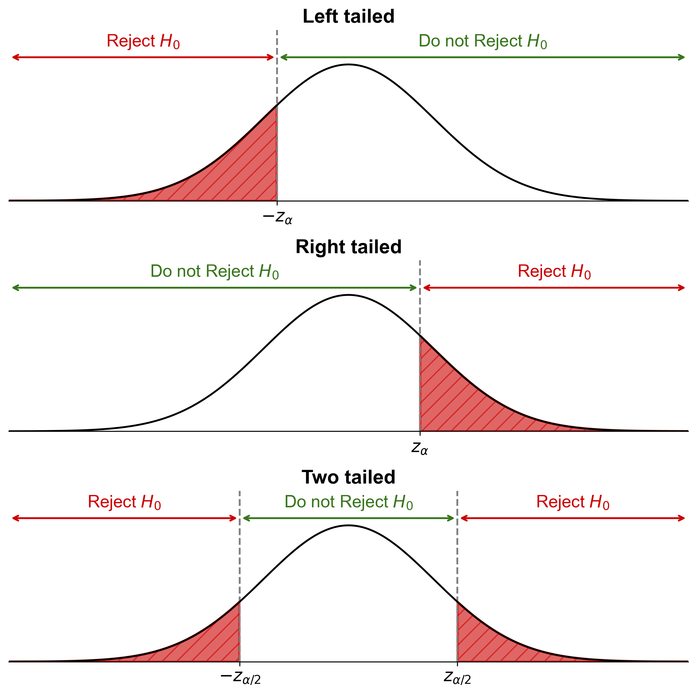
Fig. 7.1 Comparative illustration of rejection regions in hypothesis testing: Left-tailed test targets values below, right-tailed test targets values above, and two-tailed test targets values on both extremes of the hypothesized mean.#
Example 7.15
We are analyzing the effectiveness of a training program designed to improve employee productivity. After conducting the training, we calculate a test statistic, \(z = 2.5\), to assess the impact of the program on productivity scores. Given a significance level of \(\alpha = 0.05\) for a one-tail test:
a. State the null and alternative hypotheses for this test.
b. Interpret the provided test statistic \(z = 2.5\) in the context of the hypotheses.
c. Determine whether to reject or fail to reject the null hypothesis based on the provided test statistic and the significance level \(\alpha = 0.05\).
Solution:
a. Null and Alternative Hypotheses:
Null Hypothesis (\(H_0\)): The training program has no effect on employee productivity.
Alternative Hypothesis (\(H_a\)): The training program has a positive effect on employee productivity.
b. Interpretation of Test Statistic \(z = 2.5\):
The test statistic \(z = 2.5\) indicates that the sample data is 2.5 standard deviations above the mean under the null hypothesis. This suggests a significant positive effect of the training program on productivity scores.
c. Conclusion:
With a significance level \(\alpha = 0.05\), and considering this is a one-tail test, we compare the test statistic \(z = 2.5\) to the critical value \(z_{0.05} = 1.645\) (for a one-tail test at \(\alpha = 0.05\)).
Since \(z = 2.5\) is greater than \(z_{0.05} = 1.645\), we reject the null hypothesis \(H_0\).
Therefore, we conclude that the training program has a statistically significant positive effect on employee productivity based on the provided test statistic \(z = 2.5\) at the \(\alpha = 0.05\) significance level.
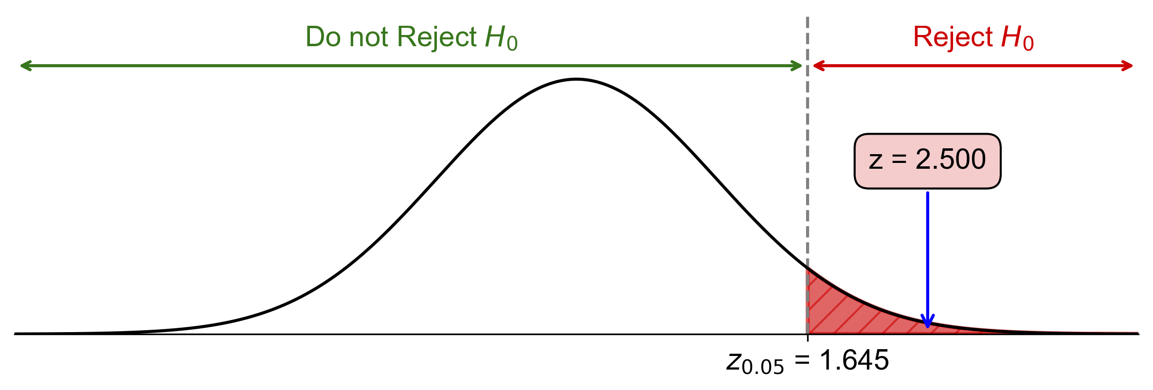
Fig. 7.2 Visualization of One-Tailed Hypothesis Test for Training Program Effectiveness#
Fig. 7.2 illustrates the one-tailed hypothesis test for this example:
The bell curve represents the standard normal distribution under the null hypothesis.
The vertical red line at \(z = 1.645\) represents the critical value for a one-tailed test at \(\alpha = 0.05\).
The shaded area to the right of the critical value represents the rejection region, which has an area of 0.05 (5%).
The vertical blue line at \(z = 2.5\) represents our calculated test statistic.
Since the blue line (our test statistic) falls within the shaded rejection region, we reject the null hypothesis.
Example 7.16
We are investigating the effect of a new study technique on exam scores. After implementing the technique, we calculate a test statistic, \(z = 1.8\), to assess its impact on exam performance. Given a significance level of \(\alpha = 0.01\) for a one-tail test:
a. State the null and alternative hypotheses for this test.
b. Interpret the provided test statistic \(z = 1.8\) in the context of the hypotheses.
c. Determine whether to reject or fail to reject the null hypothesis based on the provided test statistic and the significance level \(\alpha = 0.01\).
Solution:
a. Null and Alternative Hypotheses:
Null Hypothesis (\(H_0\)): The new study technique has no effect on exam scores.
Alternative Hypothesis (\(H_a\)): The new study technique improves exam scores.
b. Interpretation of Test Statistic \(z = 1.8\):
The test statistic \(z = 1.8\) indicates that the sample data is 1.8 standard deviations above the mean under the null hypothesis. This suggests a positive effect of the new study technique on exam performance.
c. Conclusion:
With a significance level \(\alpha = 0.01\), and considering this is a one-tail test, we compare the test statistic \(z = 1.8\) to the critical value \(z_{0.01}\).
Since the critical value \(z_{0.01}\) for a one-tail test at \(\alpha = 0.01\) is approximately \(2.33\), and \(z = 1.8\) is less than \(2.33\), we fail to reject the null hypothesis \(H_0\).
Therefore, we do not have sufficient evidence to conclude that the new study technique significantly improves exam scores based on the provided test statistic \(z = 1.8\) at the \(\alpha = 0.01\) significance level.
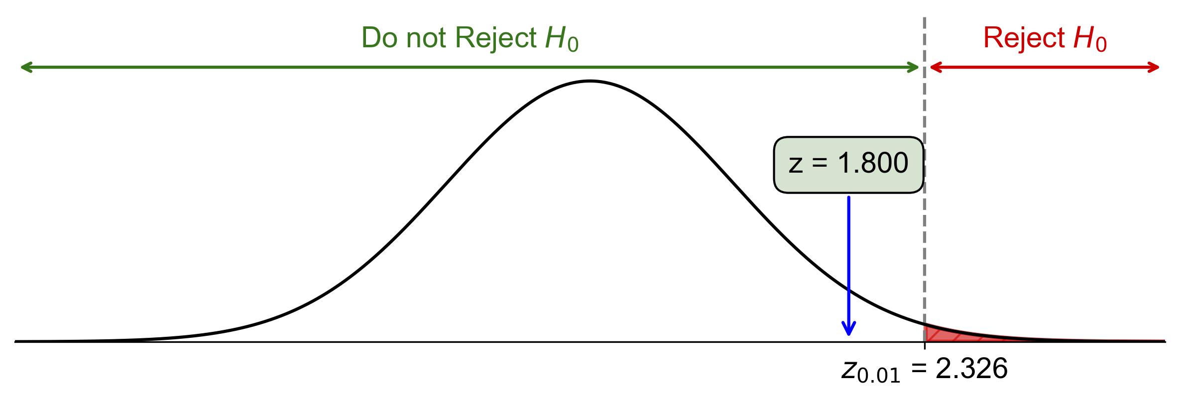
Fig. 7.3 Visualization of One-Tailed Hypothesis Test for Study Technique Effectiveness#
Fig. 7.3 illustrates the one-tailed hypothesis test for this example:
The bell curve represents the standard normal distribution under the null hypothesis.
The vertical red line at \(z = 2.326\) represents the critical value for a one-tailed test at \(\alpha = 0.01\).
The shaded area to the right of the critical value represents the rejection region, which has an area of 0.01 (1%).
The vertical blue line at \(z = 1.8\) represents our calculated test statistic.
Since the blue line (our test statistic) falls outside the shaded rejection region, we fail to reject the null hypothesis.
Example 7.17
We are investigating whether a new advertising campaign has an impact on sales conversion rates. After launching the campaign, we calculate a test statistic, \(z = -2.2\), to assess its effect. Given a significance level of \(\alpha = 0.05\) for a two-tailed test:
a. State the null and alternative hypotheses for this test.
b. Interpret the provided test statistic \(z = -2.2\) in the context of the hypotheses.
c. Determine whether to reject or fail to reject the null hypothesis based on the provided test statistic and the significance level \(\alpha = 0.05\).
Solution:
a. Null and Alternative Hypotheses:
Null Hypothesis (\(H_0\)): The new advertising campaign has no effect on sales conversion rates.
Alternative Hypothesis (\(H_a\)): The new advertising campaign has an effect on sales conversion rates.
b. Interpretation of Test Statistic \(z = -2.2\):
The test statistic \(z = -2.2\) indicates that the sample data is 2.2 standard deviations below the mean under the null hypothesis. This suggests a potential negative effect of the new advertising campaign on sales conversion rates.
c. Conclusion:
With a significance level \(\alpha = 0.05\), and considering this is a two-tailed test, we compare the absolute value of the test statistic \(|z| = 2.2\) to the critical value \(z_{0.025}\).
The critical value \(z_{0.025}\) for a two-tailed test at \(\alpha = 0.05\) is approximately \(\pm 1.96\).
Since \(|z| = 2.2\) is greater than \(1.96\), we reject the null hypothesis \(H_0\).
Therefore, we conclude that the new advertising campaign has a statistically significant effect on sales conversion rates based on the provided test statistic \(z = -2.2\) at the \(\alpha = 0.05\) significance level.
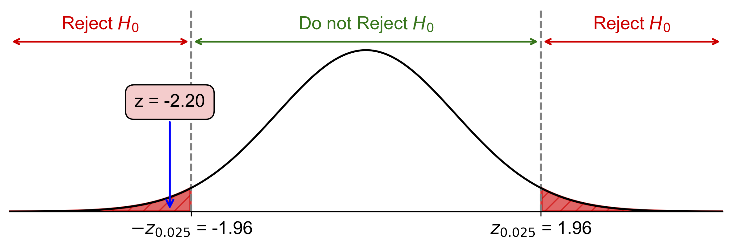
Fig. 7.4 Visualization of Two-Tailed Hypothesis Test for Advertising Campaign Effect#
Fig. 7.4 illustrates the two-tailed hypothesis test for this example:
The bell curve represents the standard normal distribution under the null hypothesis.
The vertical red lines at \(z = \pm 1.96\) represent the critical values for a two-tailed test at \(\alpha = 0.05\).
The shaded areas to the left and right of the critical values represent the rejection regions, which together have an area of 0.05 (5%).
The vertical blue line at \(z = -2.2\) represents our calculated test statistic.
Since the blue line (our test statistic) falls within the shaded rejection region on the left side, we reject the null hypothesis.
Example 7.18
We are analyzing the effect of a new medication on blood pressure. After administering the medication, we calculate a test statistic, \(z = 1.9\), to assess its impact. Given a significance level of \(\alpha = 0.01\) for a two-tailed test:
a. State the null and alternative hypotheses for this test.
b. Interpret the provided test statistic \(z = 1.9\) in the context of the hypotheses.
c. Determine whether to reject or fail to reject the null hypothesis based on the provided test statistic and the significance level \(\alpha = 0.01\).
Solution:
a. Null and Alternative Hypotheses:
Null Hypothesis (\(H_0\)): The new medication has no effect on blood pressure.
Alternative Hypothesis (\(H_a\)): The new medication has an effect on blood pressure.
b. Interpretation of Test Statistic \(z = 1.9\):
The test statistic \(z = 1.9\) indicates that the sample data is 1.9 standard deviations above the mean under the null hypothesis. This suggests a potential positive effect of the new medication on blood pressure.
c. Conclusion:
With a significance level \(\alpha = 0.01\), and considering this is a two-tailed test, we compare the absolute value of the test statistic \(|z| = 1.9\) to the critical value \(z_{0.005}\).
The critical value \(z_{0.005}\) for a two-tailed test at \(\alpha = 0.01\) is approximately \(\pm 2.58\).
Since \(|z| = 1.9\) is less than \(2.58\), we fail to reject the null hypothesis \(H_0\).
Therefore, we do not have sufficient evidence to conclude that the new medication has a statistically significant effect on blood pressure based on the provided test statistic \(z = 1.9\) at the \(\alpha = 0.01\) significance level.
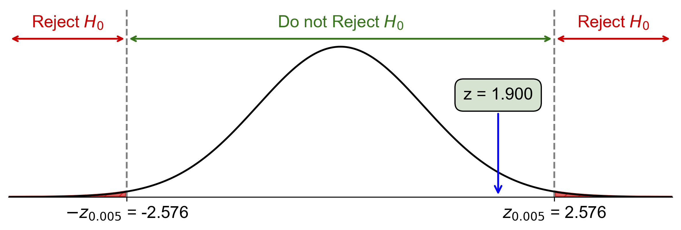
Fig. 7.5 Visualization of Two-Tailed Hypothesis Test for Blood Pressure Medication Effect#
Fig. 7.5 illustrates the two-tailed hypothesis test for this example:
The bell curve represents the standard normal distribution under the null hypothesis.
The vertical red lines at \(z = \pm 2.576\) represent the critical values for a two-tailed test at \(\alpha = 0.01\).
The shaded areas to the left and right of the critical values represent the rejection regions, which together have an area of 0.01 (1%).
The vertical blue line at \(z = 1.9\) represents our calculated test statistic.
Since the blue line (our test statistic) falls outside the shaded rejection regions, we fail to reject the null hypothesis.
Example 7.19
We are investigating whether a new manufacturing process reduces defect rates. After implementing the process, we calculate a test statistic, \(z = -1.8\), to assess its effect. Given a significance level of \(\alpha = 0.05\) for a left-tailed test:
a. State the null and alternative hypotheses for this test.
b. Interpret the provided test statistic \(z = -1.8\) in the context of the hypotheses.
c. Determine whether to reject or fail to reject the null hypothesis based on the provided test statistic and the significance level \(\alpha = 0.05\).
Solution:
a. Null and Alternative Hypotheses:
Null Hypothesis (\(H_0\)): The new manufacturing process has no effect on defect rates.
Alternative Hypothesis (\(H_a\)): The new manufacturing process reduces defect rates.
b. Interpretation of Test Statistic \(z = -1.8\):
The test statistic \(z = -1.8\) indicates that the sample data is 1.8 standard deviations below the mean under the null hypothesis. This suggests a potential reduction in defect rates due to the new manufacturing process.
c. Conclusion:
With a significance level \(\alpha = 0.05\), and considering this is a left-tailed test, we compare the test statistic \(z = -1.8\) to the critical value \(z_{0.05}\).
The critical value \(z_{0.05}\) for a left-tailed test at \(\alpha = 0.05\) is approximately \(-1.645\).
Since \(z = -1.8\) is less than \(-1.645\), we reject the null hypothesis \(H_0\).
Therefore, we conclude that the new manufacturing process has a statistically significant effect in reducing defect rates based on the provided test statistic \(z = -1.8\) at the \(\alpha = 0.05\) significance level.
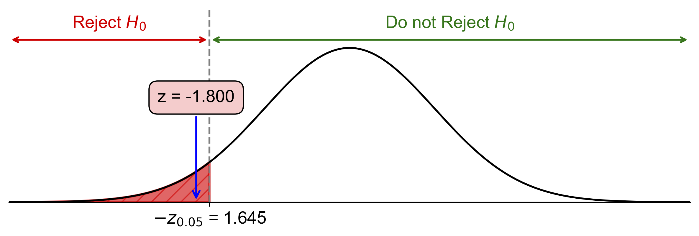
Fig. 7.6 Visualization of Left-Tailed Hypothesis Test for Manufacturing Process Effect#
Fig. 7.6 illustrates the left-tailed hypothesis test for this example:
The bell curve represents the standard normal distribution under the null hypothesis.
The vertical red line at \(z = -1.645\) represents the critical value for a left-tailed test at \(\alpha = 0.05\).
The shaded area to the left of the critical value represents the rejection region, which has an area of 0.05 (5%).
The vertical blue line at \(z = -1.8\) represents our calculated test statistic.
Since the blue line (our test statistic) falls within the shaded rejection region, we reject the null hypothesis.
Example 7.20
We are analyzing whether a new treatment decreases recovery time for patients. After administering the treatment, we calculate a test statistic, \(z = -2.3\), to assess its effect. Given a significance level of \(\alpha = 0.01\) for a left-tailed test:
a. State the null and alternative hypotheses for this test.
b. Interpret the provided test statistic \(z = -2.3\) in the context of the hypotheses.
c. Determine whether to reject or fail to reject the null hypothesis based on the provided test statistic and the significance level \(\alpha = 0.01\).
Solution:
a. Null and Alternative Hypotheses:
Null Hypothesis (\(H_0\)): The new treatment has no effect on recovery time.
Alternative Hypothesis (\(H_a\)): The new treatment decreases recovery time.
b. Interpretation of Test Statistic \(z = -2.3\):
The test statistic \(z = -2.3\) indicates that the sample data is 2.3 standard deviations below the mean under the null hypothesis. This suggests a potential decrease in recovery time due to the new treatment.
c. Conclusion:
With a significance level \(\alpha = 0.01\), and considering this is a left-tailed test, we compare the test statistic \(z = -2.3\) to the critical value \(z_{0.01}\).
The critical value \(z_{0.01}\) for a left-tailed test at \(\alpha = 0.01\) is approximately \(-2.33\).
Since \(z = -2.3\) is greater than \(-2.33\), we fail to reject the null hypothesis \(H_0\).
Therefore, we do not have sufficient evidence to conclude that the new treatment has a statistically significant effect in decreasing recovery time based on the provided test statistic \(z = -2.3\) at the \(\alpha = 0.01\) significance level.
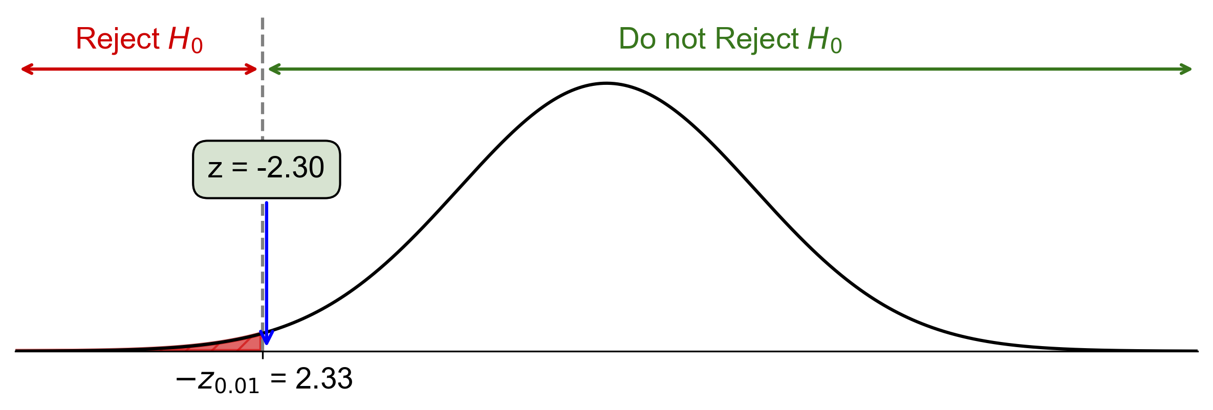
Fig. 7.7 Visualization of Left-Tailed Hypothesis Test for Treatment Effect on Recovery Time#
Fig. 7.7 illustrates the left-tailed hypothesis test for this example:
The bell curve represents the standard normal distribution under the null hypothesis.
The vertical red line at \(z = -2.33\) represents the critical value for a left-tailed test at \(\alpha = 0.01\).
The shaded area to the left of the critical value represents the rejection region, which has an area of 0.01 (1%).
The vertical blue line at \(z = -2.3\) represents our calculated test statistic.
Since the blue line (our test statistic) falls outside the shaded rejection region, we fail to reject the null hypothesis.
