5.5. The Lognormal Distribution

The Log-normal Distribution is particularly useful for modeling data that are highly skewed or contain outliers. Unlike the normal distribution, which may not adequately capture the characteristics of such data, the log-normal distribution often provides a better fit due to its inherent skewness.

5.5.1. Relationship to the Normal Distribution

• Consider a normal random variable, \(X\), with mean \(\mu\) and variance \(\sigma^2\).

• If we take the exponential of \(X\), denoted as \(Y = e^X\), the resulting random variable \(Y\) follows a log-normal distribution.

• Thus, if \(X \sim N(\mu, \sigma^2)\), then \(Y = e^X\) follows a log-normal distribution with the same parameters \(\mu\) and \(\sigma^2\).

Conversely:

• If \(Y\) is log-normally distributed with parameters \(\mu\) and \(\sigma^2\), then \(X = \ln(Y)\) will follow a normal distribution with mean \(\mu\) and variance \(\sigma^2\).

5.5.2. Probability Density Function (PDF)

The probability density function (PDF) of a log-normal random variable is:

\[\begin{equation*} f(x) = \begin{cases}\dfrac{1}{x\sigma\sqrt{2\pi}} \exp\left(-\dfrac{1}{2\sigma^2} (\ln(x) - \mu)^2\right) & \text{if } x > 0 \\ & \\ 0 & \text{if } x \leq 0 \end{cases} \end{equation*}\]

This function is defined for \(x > 0\) and highlights the skewness of the log-normal distribution. This skewness makes it suitable for modeling processes that produce occasional large values, such as outliers.

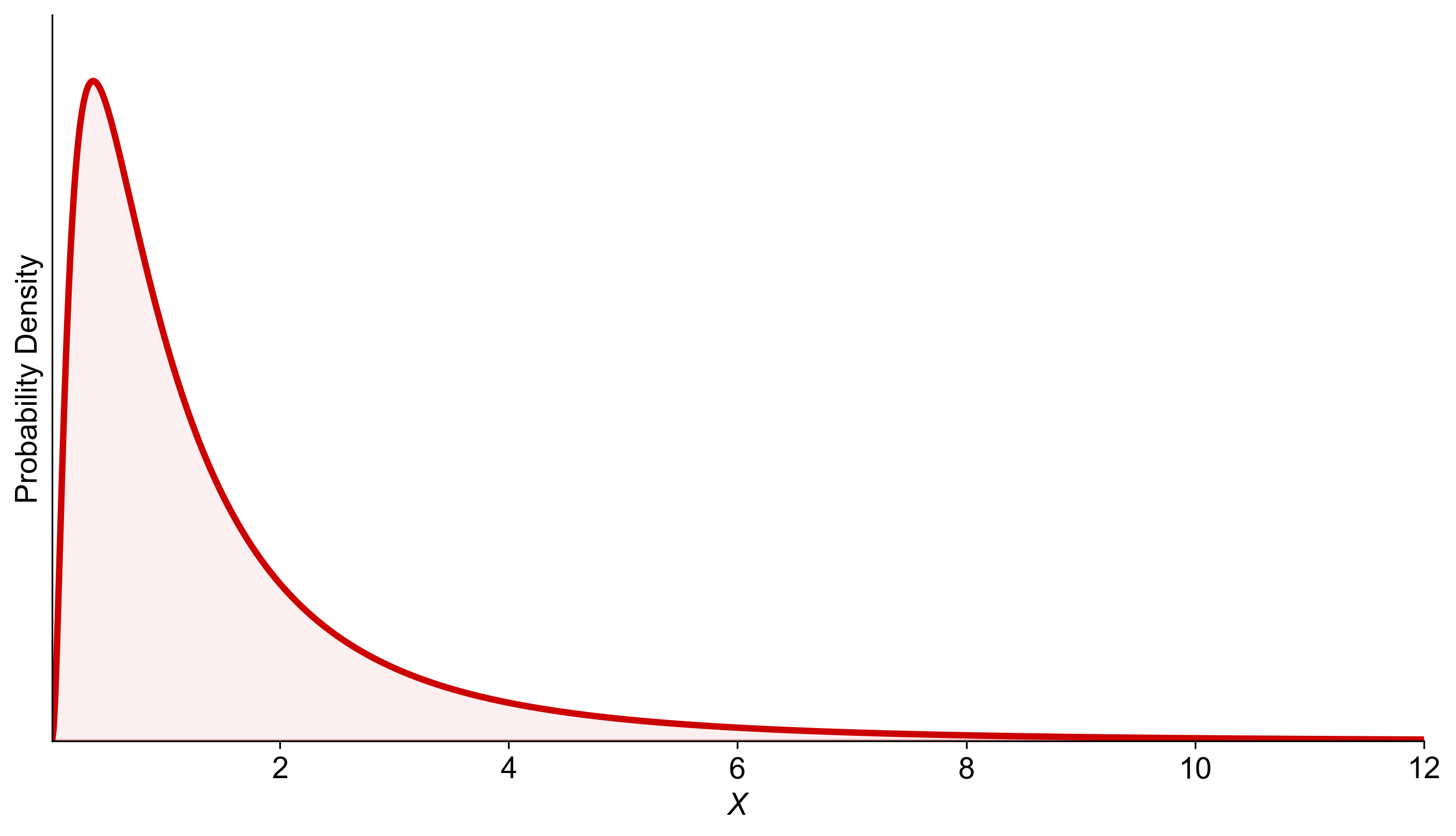
For example, with parameters \(\mu = 0\) and \(\sigma = 1\), the graph of this PDF would show a significant skew to the right, indicating that while most values are clustered around the lower end, there’s a long tail towards the higher values, representing the potential for outliers. This characteristic is what makes the lognormal distribution a powerful tool for modeling certain types of data.

Fig. 5.21 illustrates the probability density function (PDF) of a lognormal distribution with parameters \(\mu = 0\) and \(\sigma = 1\). The curve starts high near the vertical axis and sharply declines, creating a long tail to the right, indicating a right-skewed distribution. This shape shows that lower values of \(X\) have higher probabilities, while higher values are less likely but possible, representing outliers.

Fig. 5.53 Probability density function of the lognormal distribution with \(\mu = 0\) and \(\sigma = 1\), highlighting its right-skewed nature and suitability for data with outliers.

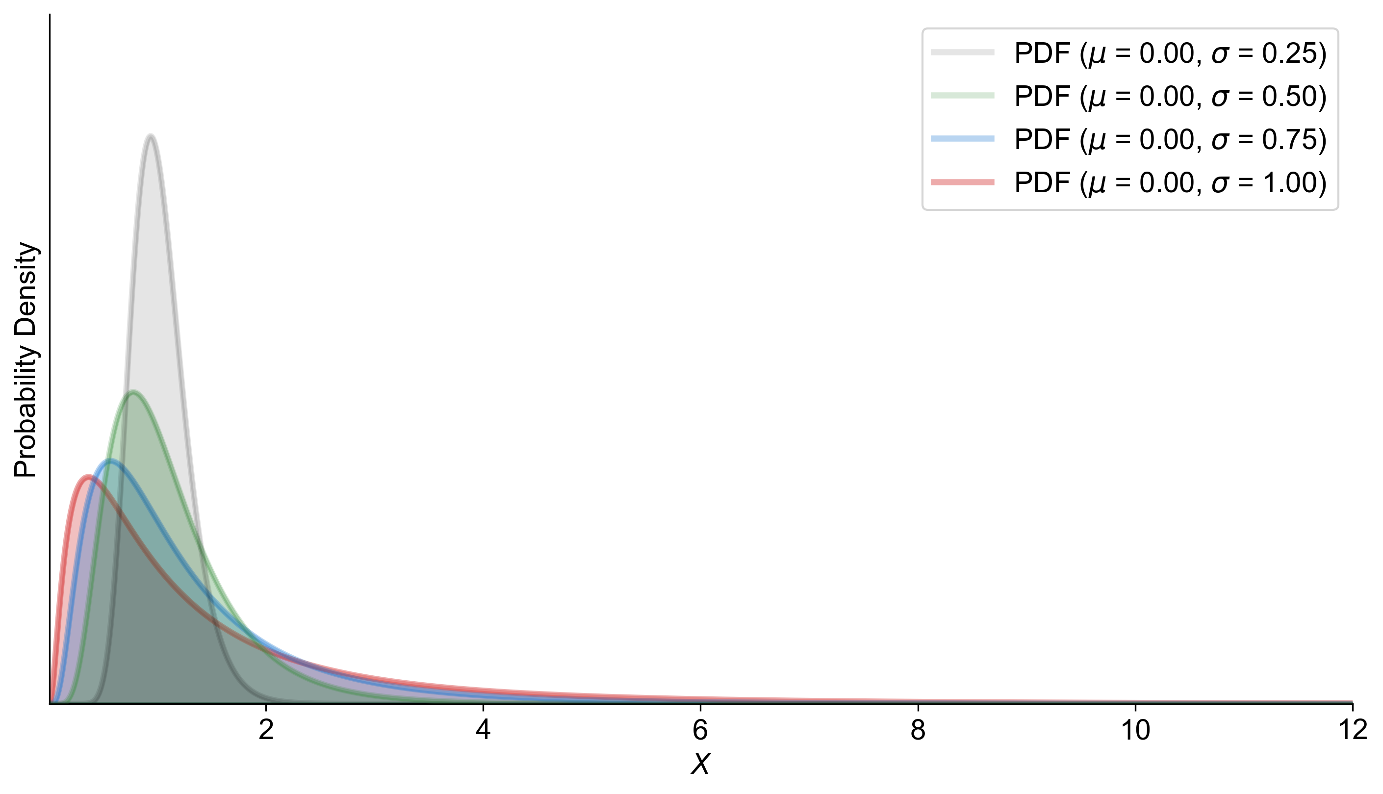
Fig. 5.54 displays the probability density functions (PDFs) of lognormal distributions with a mean (μ) of 0 and varying standard deviations (σ). The curves are color-coded for clarity:

• Red Curve: σ = 1.00

• Blue Curve: σ = 0.75

• Green Curve: σ = 0.50

• Black Curve: σ = 0.25

As the standard deviation decreases, the peak of the curve becomes higher and narrower, indicating less variability around the mean. Conversely, a higher standard deviation results in a lower and wider peak, showing more spread in the data. This visualization helps in understanding how the spread of data changes with different standard deviations in a lognormal distribution.

Fig. 5.54 Probability density functions of lognormal distributions with different standard deviations.

The standard lognormal distribution is a probability distribution that’s skewed to the right, making it suitable for modeling data that can exhibit large, atypical values. It’s derived from the normal distribution through a transformation process. Specifically, if a variable \( X \) follows a normal distribution with a mean (\( \mu \)) of 0 and a standard deviation (\( \sigma \)) of 1, then the exponential of \( X \), denoted as \( Y = e^X \), will follow a standard lognormal distribution.

In this context:

• The mean (\( \mu \)) on the normal scale is 0, which after transformation becomes the scale parameter \( e^\mu = 1 \) for the lognormal distribution.

• The standard deviation (\( \sigma \)), which measures the spread of data on the normal scale, remains unchanged during the transformation and continues to shape the lognormal distribution.

The resulting graph of the lognormal density function, with these parameters, shows a pronounced rightward skew. This characteristic is why the lognormal distribution is frequently used in scenarios where data are expected to have occasional extreme values, also known as outliers. Such data sets are common in fields like finance, insurance, and environmental studies, where they help in modeling phenomena like stock prices, claim sizes, or pollutant concentrations, respectively.

5.5.3. Mean and Variance of a Log-normal Random Variable

If \( Y \) is a lognormal random variable with parameters \(\mu\) and \(\sigma^2\), advanced methods can show that its mean \(E(Y)\) and variance \(V(Y)\) are given by:

(5.21)\[\begin{equation} E(Y) = e^{\mu + \sigma^2 / 2} \end{equation}\]

(5.22)\[\begin{equation} V(Y) = e^{2\mu + 2\sigma^2} - e^{2\mu + \sigma^2} \end{equation}\]

It is important to note that for a lognormal distribution, the parameters \(\mu\) and \(\sigma^2\) do not represent the mean and variance of \(Y\). Instead, they are the mean and variance of the normally distributed variable \(\ln Y\). The notation \(E(Y)\) is used instead of \(\mu_Y\), and \(V(Y)\) is used instead of \(\sigma_Y^2\), to prevent confusion with the parameters \(\mu\) and \(\sigma\).

Example 5.21

The lifetimes of a particular type of battery are lognormally distributed with parameters \( \mu = 0.5 \) days and \( \sigma = 0.25 \) days. Calculate the mean lifetime of these batteries. Also, find the standard deviation of the lifetimes.

Solution:

Let \( Z \) represent the lifetime of a randomly selected battery. To find the mean lifetime of the batteries, we use the formula for the mean of a lognormal distribution:

\[\begin{equation*}\text{Mean} = e^{\mu + \dfrac{\sigma^2}{2}}\end{equation*}\]

Substituting the given values:

\[\begin{equation*}\text{Mean} = e^{0.5 + \dfrac{0.25^2}{2}} = e^{0.5 + 0.03125} = e^{0.53125}\end{equation*}\]

Calculating the exponent:

\[\begin{equation*}\text{Mean} \approx e^{0.53125} \approx 1.7011 \text{ days}\end{equation*}\]

Next, we find the variance using the formula for the variance of a lognormal distribution:

\[\begin{equation*}\text{Variance} = (e^{\sigma^2} - 1) \cdot e^{2\mu + \sigma^2}\end{equation*}\]

Substituting the given values:

\[\begin{equation*}\text{Variance} = (e^{0.25^2} - 1) \cdot e^{2 \cdot 0.5 + 0.25^2} = (e^{0.0625} - 1) \cdot e^{1.0625}\end{equation*}\]

Calculating the variance:

\[\begin{equation*}\text{Variance} \approx (e^{0.0625} - 1) \cdot e^{1.0625} \approx 0.1866\end{equation*}\]

Finally, the standard deviation is the square root of the variance:

\[\begin{equation*}\text{Standard Deviation} = \sqrt{0.1866} \approx 0.4320 \text{ days}\end{equation*}\]

So, the mean lifetime of the batteries is approximately 1.7011 days, and the standard deviation of the lifetimes is approximately 0.4320 days. These calculations assume that the lifetimes follow a lognormal distribution with the specified parameters. Remember, the actual values may vary slightly due to rounding during the calculation process.

5.5.4. Assessing Data for Lognormal Distribution

When evaluating data sets, especially those that are skewed or contain extreme values, it’s crucial to determine the appropriate statistical distribution. Unlike data from a normal distribution, which seldom have outliers, lognormal data often exhibit a few significantly larger values due to the characteristic long right-hand tail of the lognormal distribution.

To ascertain if a data set originates from a lognormal distribution, a common approach is to apply a logarithmic transformation to each data point. If the resulting transformed data set resembles a normal distribution, it suggests that the original data may indeed be lognormal.

5.5.5. Characteristics of Lognormal Distributions

• Pronounced right-hand tail: This leads to outliers predominantly on the higher end.

• Unsuitability for extremely low values: Lognormal distributions do not accommodate negative numbers or zero.

• Exclusivity to positive values: The logarithm of non-positive numbers is undefined.

It’s important to recognize that a logarithmic transformation does not guarantee a normal distribution approximation. To confirm, one should create and analyze a histogram or probability plot of the transformed data.

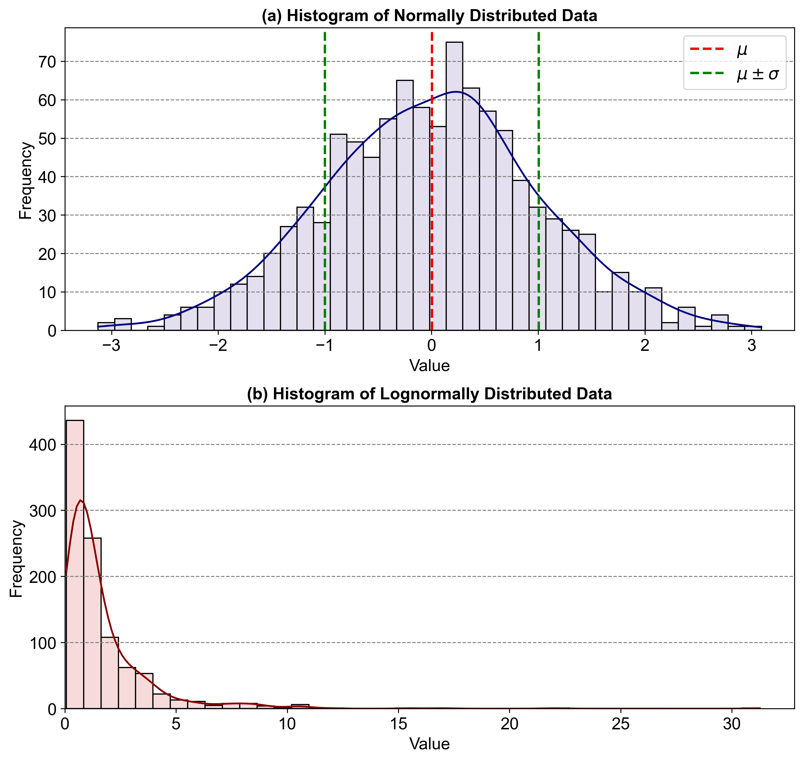
Fig. 5.53 contains two histograms illustrating the characteristics of normally distributed data and lognormally distributed data:

• Histogram (a): Shows normally distributed data with a bell-shaped curve. The red line indicates the mean, while the green dashed lines represent one standard deviation from the mean.

• Histogram (b): Displays lognormally distributed data with a pronounced right-hand tail, indicating the presence of outliers on the higher end. This skewness is characteristic of lognormal distributions, which are suitable for modeling data with extreme values.

Fig. 5.55 Comparison of Normally and Lognormally Distributed Data: (a) Normally distributed data with a bell-shaped curve and (b) Lognormally distributed data with a pronounced right-hand tail.

Example 5.22

A machine produces bolts whose lengths are lognormally distributed. If the lengths of these bolts have parameters \(\mu = 2.5\) mm and \(\sigma = 0.3\) mm, calculate the mean length and the standard deviation of the lengths of these bolts.

Solution: The mean length of the bolts is given by:

\[\begin{equation*}\text{Mean} = e^{\mu + \dfrac{\sigma^2}{2}}\end{equation*}\]

Substituting the given values:

\[\begin{equation*}\text{Mean} = e^{2.5 + \dfrac{0.3^2}{2}} \approx e^{2.545} \approx 12.7432 \text{ mm}\end{equation*}\]

The variance of the lengths is given by:

\[\begin{equation*}\text{Variance} = (e^{\sigma^2} - 1) \cdot e^{2\mu + \sigma^2}\end{equation*}\]

Substituting the given values:

\[\begin{equation*}\text{Variance} = (e^{0.3^2} - 1) \cdot e^{2 \cdot 2.5 + 0.3^2} \approx 15.2929 \text{ mm}^2\end{equation*}\]

The standard deviation is the square root of the variance:

\[\begin{equation*}\text{Standard Deviation} = \sqrt{15.2929} \approx 3.9106 \text{ mm}\end{equation*}\]

Therefore, the mean length of the bolts is approximately 12.7432 mm, and the standard deviation of the lengths is approximately 3.9106 mm.

Example 5.23

The weight of a certain breed of dogs is lognormally distributed. Given that the parameters for this distribution are \(\mu = 1\) kg and \(\sigma = 0.2\) kg, find the probability that a randomly selected dog from this breed weighs more than 3 kg.

Solution: First, we calculate the z-score for 3 kg using the formula for a lognormal distribution:

\[\begin{equation*}z = \dfrac{\ln(3) - \mu}{\sigma}\end{equation*}\]

Substituting the given values:

\[\begin{equation*}z = \dfrac{\ln(3) - 1}{0.2} \approx 0.49\end{equation*}\]

Now, we find the probability that a dog weighs more than 3 kg by subtracting the cumulative distribution function (CDF) value for this z-score from 1:

\[\begin{equation*}P(X > 3) = 1 - \text{CDF}(0.49)\end{equation*}\]

Using a standard normal distribution table or a calculator, we find:

\[\begin{equation*}P(X > 3) \approx 1 - 0.6890 \approx 0.3110\end{equation*}\]

Therefore, there is approximately a 31.10% chance that a randomly selected dog from this breed weighs more than 3 kg.

This correction aligns with the output of your Python code, providing the accurate probability for the given scenario.