Hypothesis Testing of a Single Mean

7.6. Hypothesis Testing of a Single Mean#

7.6.1. Choosing the Hypotheses#

The null hypothesis (\(H_0\)) is a statement or claim that is assumed to be true or represents the status quo, often based on prior knowledge, previous research, or conventional wisdom. It serves as a starting point for hypothesis testing, where we want to determine if there is enough evidence to reject H0 and accept an alternative hypothesis (\(H_a\)) that contradicts \(H_0\). The alternative hypothesis (\(H_a\)), on the other hand, is the claim that researchers want to support or demonstrate as true. It represents the possibility that there is a meaningful effect or relationship in the population being studied.

In hypothesis testing, we collect sample data and perform statistical analyses to assess whether the evidence from the sample supports the alternative hypothesis (\(H_a\)) or if it is more in line with the null hypothesis (\(H_0\)). The process involves comparing the observed data with what we would expect to see if \(H_0\) were true.

If the sample evidence provides strong enough support against the null hypothesis (\(H_0\)), we reject it in favor of the alternative hypothesis (\(H_a\)). This indicates that there is sufficient evidence to suggest that the alternative hypothesis is likely true or represents a more accurate explanation of the phenomenon being studied.

On the other hand, if the sample evidence does not provide enough support to contradict the null hypothesis (\(H_0\)), we fail to reject it. This means that there is not enough evidence to suggest that the alternative hypothesis is more plausible, and we may continue to believe in the validity of the null hypothesis.

In summary, the two possible conclusions from a hypothesis-testing analysis are:

Reject \(H_0\): If the sample evidence strongly contradicts the null hypothesis (\(H_0\)), we reject \(H_0\) in favor of the alternative hypothesis (\(H_a\)).
Fail to reject \(H_0\): If the sample evidence does not strongly contradict the null hypothesis (\(H_0\)), we do not have enough evidence to support the alternative hypothesis (\(H_a\)), and we continue to believe in the plausibility of \(H_0\). It does not necessarily mean that \(H_0\) is proven to be true; it only means that we have not found enough evidence to reject it at the given level of significance.

7.6.2. Null Hypothesis for Population Mean#

The null hypothesis for a hypothesis test concerning a population mean (\(\mu\)) specifies a single value for that parameter. This value serves as the point of reference for the hypothesis test.

For a population mean (\(\mu\)), the null hypothesis can take one of the following forms:

a. \(H_0: \mu = \mu_{0}\) (The population mean is equal to a specific value, \(\mu_{0}\)).
b. \(H_0: \mu \geq \mu_{0}\) (The population mean is greater than or equal to a certain value, \(\mu_{0}\)).
c. \(H_0: \mu \leq \mu_{0}\) (The population mean is less than or equal to a certain value, \(\mu_{0}\)).

Here, \(\mu_{0}\) represents the fixed numerical value that serves as the reference point for the hypothesis test.

7.6.3. Alternative Hypothesis for Population Mean#

The alternative hypothesis for a hypothesis test concerning a population mean (\(\mu\)) follows a specific pattern, corresponding to the type of test being conducted. Here are the forms for each type of test:

Two-Tailed Test: If the primary concern is to determine whether a population mean, \(\mu\), is different from a specified value \(\mu_{0}\), the alternative hypothesis is expressed as:

(7.9)#\[\begin{equation} H_a: \mu \neq \mu_{0} \end{equation}\]

A hypothesis test with this form of the alternative hypothesis is referred to as a two-tailed test. In this test, we are interested in detecting any significant difference between the population mean and the specified value, without specifying whether it is greater or lesser.

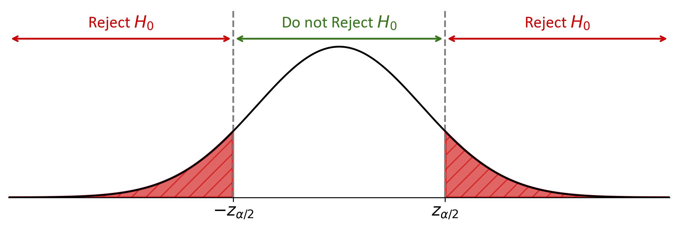
Fig. 7.21 illustrates a hypothesis test using a normal distribution curve. The bell-shaped curve is centered on the mean, marked by a vertical dashed line. The shaded red areas to both the left and right of this line represent the critical regions starting at “\(-z_{\alpha/2}\)” and “\(z_{\alpha/2}\)” on the horizontal axis. If a test statistic falls within either of these shaded areas, the null hypothesis (\(H_0\)) should be rejected. The unshaded area in the middle indicates where the null hypothesis would not be rejected. This visual helps in understanding the placement of a test statistic relative to the critical values and its implications for the hypothesis test.

../_images/hypothesis_test_two_tail.jpg — Fig. 7.21 Normal Distribution Curve Highlighting Critical Regions for Hypothesis Testing: The shaded areas under the curve on both sides of the mean represent the critical regions for rejecting the null hypothesis, while the central area indicates acceptance of the null hypothesis.#

Left-Tailed Test: If the main interest is to decide whether a population mean, \(\mu\), is less than a specified value \(\mu_{0}\), the alternative hypothesis is expressed as:

(7.10)#\[\begin{equation} H_a: \mu < \mu_{0} \end{equation}\]

A hypothesis test with this form of the alternative hypothesis is called a left-tailed test. Here, the focus is on identifying whether the population mean is significantly smaller than the specified value.

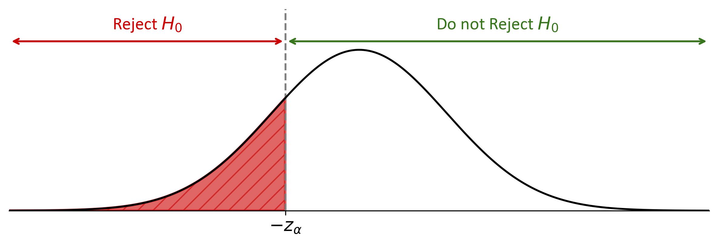
Fig. 7.22 illustrates a hypothesis test using a normal distribution curve. The bell-shaped curve is centered on the mean, marked by a vertical dashed line. The shaded red area to the left of this line represents the critical region starting at “\(-z_{\alpha}\)” on the horizontal axis. If a test statistic falls within this shaded area, the null hypothesis (\(H_0\)) should be rejected. The unshaded area to the right indicates where the null hypothesis would not be rejected. This visual helps in understanding the placement of a test statistic relative to the critical value and its implications for the hypothesis test.

../_images/hypothesis_test_left_tail.jpg — Fig. 7.22 Normal Distribution Curve Highlighting Critical Regions for Hypothesis Testing: The shaded area under the curve to the left of the mean represents the critical region for rejecting the null hypothesis, while the area to the right indicates acceptance of the null hypothesis.#

Right-Tailed Test: If the primary concern is to determine whether a population mean, \(\mu\), is greater than a specified value \(\mu_{0}\), the alternative hypothesis is expressed as:

(7.11)#\[\begin{equation} H_a: \mu > \mu_{0} \end{equation}\]

A hypothesis test with this form of the alternative hypothesis is referred to as a right-tailed test. The emphasis here is on detecting whether the population mean is significantly greater than the specified value.

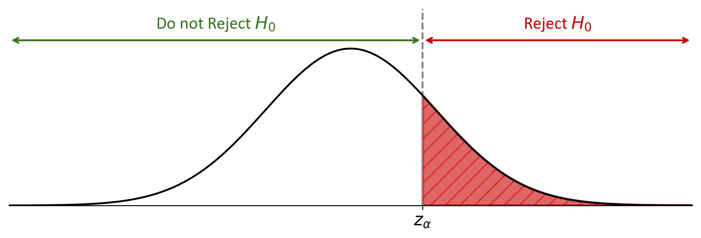
Fig. 7.23 illustrates a hypothesis test using a normal distribution curve. The bell-shaped curve is centered on the mean, marked by a vertical dashed line. The shaded red area to the right of this line represents the critical region starting at “\(z_{\alpha}\)” on the horizontal axis. If a test statistic falls within this shaded area, the null hypothesis (\(H_0\)) should be rejected. The unshaded area to the left indicates where the null hypothesis would not be rejected. This visual helps in understanding the placement of a test statistic relative to the critical value and its implications for the hypothesis test.

../_images/hypothesis_test_right_tail.jpg — Fig. 7.23 Normal Distribution Curve Highlighting Critical Regions for Hypothesis Testing: The shaded area under the curve to the right of the mean represents the critical region for rejecting the null hypothesis, while the area to the left indicates acceptance of the null hypothesis.#

In each case, \(\mu_{0}\) represents the specific value against which the test is being conducted. The choice of the alternative hypothesis—whether two-tailed, left-tailed, or right-tailed—depends on the research question and what the investigator seeks to establish through the hypothesis test. The appropriate choice ensures that the hypothesis test aligns with the specific objective of the study.

A summary of the above discussion is available at Table 7.3.

Table 7.3 Null and alternative hypotheses for population mean and proportion tests.#
Test Type	Population Mean (\(\mu\))
Two-Tailed Test	\(H_0\): \(\mu = \mu_{0}\) \(H_a\): \(\mu \neq \mu_{0}\)
Left-Tailed Test	\(H_0\): \(\mu \geq \mu_{0}\) \(H_a\): \(\mu < \mu_{0}\)
Right-Tailed Test	\(H_0\): \(\mu \leq \mu_{0}\) \(H_a\): \(\mu > \mu_{0}\)

Notes

A hypothesis test is called a one-tailed test if it is either left-tailed or right-tailed.
The null hypothesis (\(H_0\)) will always have an equal sign (either =, \(\leq\), or \(\geq\)). The alternative hypothesis contains values that are alternatives to those specified in \(H_0\).

7.6.4. Distribution Needed for Hypothesis Testing of Population Mean#

In Section 5.6, we learned about sampling distributions, which are essential for hypothesis testing. Depending on the situation and the available information, different distributions are associated with specific hypothesis tests:

a) When the population standard deviation is known or the sample size is large (usually \(n > 30\)), we use a normal distribution to perform hypothesis tests for a population mean.
b) When the population standard deviation is unknown and the sample size is relatively small (usually \(n \leq 30\)), we utilize a Student’s t-distribution to conduct hypothesis tests for a population mean. The t-distribution accounts for the added uncertainty when estimating the population standard deviation from a small sample.

7.6.5. Tests of Population Mean When Population Standard Deviation Is Known#

When conducting a hypothesis test for a single population mean with a known population standard deviation, the distribution used for the test is the distribution of sample means:

(7.12)#\[\begin{equation} \overline{X} \sim N\left( \mu_{X}, \dfrac{\sigma_{X}}{\sqrt{n}} \right) \end{equation}\]

where:

\(\overline{X}\) represents the sample mean.
\(\mu_{X}\) is the population mean (the parameter being tested).
\(\sigma_{X}\) denotes the population standard deviation.
\(n\) represents the sample size.

If the population standard deviation \(\sigma_{X}\) is known, the sampling distribution of the sample mean \(\overline{X}\) is a normal distribution with mean \(\mu_{X}\) and standard deviation \(\dfrac{\sigma_{X}}{\sqrt{n}}\).

Note

We will discuss this in Section 7.7.

7.6.6. Tests of Population Mean When Population Standard Deviation Is Unknown#

When the population standard deviation \(\sigma_{X}\) is unknown and the sample size is relatively small (usually \(n \leq 30\)), we use a Student’s t-distribution to conduct hypothesis tests for a population mean. The t-distribution accounts for the additional uncertainty introduced by estimating the population standard deviation from the sample:

(7.13)#\[\begin{equation} \overline{X} \sim t\left( \mu_{X}, \dfrac{s_{X}}{\sqrt{n}}, df \right) \end{equation}\]

where:

\(\overline{X}\) represents the sample mean.
\(\mu_{X}\) is the population mean (the parameter being tested).
\(s_{X}\) denotes the sample standard deviation.
\(n\) represents the sample size.
\(df\) (degrees of freedom) is \(n - 1\).

In this context, \(\overline{x}\) serves as the point estimate for the population mean \(\mu\), obtained from the sample mean \(\overline{X}\).

Note

We will discuss this in Section 7.8.