5.6. Sampling Distributions and Estimators

5.6.1. Population Parameter and a Sample Statistic.

A parameter is a value that describes a characteristic of a population, such as the population mean, while a statistic is a value that describes a characteristic of a sample, such as the sample mean.

Table 5.1 illustrates the differences between sample statistics and population parameters across various contexts, highlighting how specific samples can provide insights into broader populations.

Table 5.1 Comparison of Sample Statistics and Population Parameters

Sample statistic	Population parameter
Proportion of 2000 randomly sampled participants that support free tuition for universities.	Proportion of all Canadian residents that support free tuition for universities.
Median income of 850 college students in Calgary and Edmonton.	Median income of all college students in Alberta.
Standard deviation of weights of apples from one farm.	Standard deviation of weights of all apples in the region.
Mean screen time of 3000 high school students in Vancouver.	Mean screen time of all high school students in British Columbia.

The sampling distribution of a statistic is a concept in statistics that helps us understand the behavior of a specific statistic (e.g., sample proportion or sample mean) when we take multiple random samples from a population.

To illustrate this concept, let’s focus on the sample mean as an example. The sample mean is calculated by taking the sum of all values in a sample and dividing it by the sample size. Now, imagine that we have a population with known characteristics, such as a population of heights of all adults in a particular city.

The sampling distribution of the sample mean would involve taking multiple random samples (all of the same size, denoted as \(n\) from this population. Each sample is obtained by randomly selecting \(n\) individuals from the population and calculating the mean of that particular sample.

Now, if we repeat this process many times and collect the means of all these samples, we would end up with a distribution of sample means. This distribution is what we call the sampling distribution of the sample mean. Each value in this distribution represents the mean of a different random sample taken from the population.

Key points about the sampling distribution of a statistic

1. Center: The center of the sampling distribution is expected to be very close to the population parameter (the mean of the population). In the case of the sample mean, the center of the sampling distribution would be approximately equal to the population mean.

2. Shape: Under certain conditions (e.g., the sample size is reasonably large), the sampling distribution tends to be approximately normally distributed. This is known as the Central Limit Theorem, and it is essential in many statistical analyses.

3. Spread: The spread of the sampling distribution (i.e., its variability) is related to the sample size \(n\) A larger sample size typically results in a smaller spread, meaning that the sample mean is more likely to be close to the population mean.

4. Standard Error: The standard error of the statistic (e.g., standard error of the sample mean) is a measure of the spread of the sampling distribution. It quantifies the typical distance between the sample statistic and the population parameter.

The sampling distribution helps us make inferences about the population based on sample data. It allows us to estimate the population parameter (e.g., population mean) and make statements about the precision of our estimates using measures like confidence intervals.

Overall, understanding the concept of sampling distribution is crucial for statisticians and researchers to draw meaningful conclusions from their data and make accurate inferences about the populations they are studying.

Definition - Sampling Distribution of a Statistic

The sampling distribution of a statistic, such as a sample proportion or sample mean, represents the distribution of that statistic when all possible samples of the same size (\(n\)) are drawn from the same population. This distribution is often illustrated as a probability histogram, formula, or table, showing the probabilities associated with various values of the statistic. It provides valuable insights into the variability and characteristics of the statistic, aiding in making inferences about the underlying population.

Note

\(\widehat{p}\) is pronounced “p-hat.” When symbols are used above a letter, as in \(\bar{x}\) and \(\widehat{p},\) they represent statistics, not parameters.

Table 5.2 provides a clear comparison between common sample statistics and their corresponding population parameters, using standard notations and terminology.

Table 5.2 Comparison of Sample Statistics and Population Parameters Terminologies

	Sample statistic	Population parameter
Proportion	\(\widehat{p}\) (called “p-hat”)	\(p\)
Mean	\(\overline{x}\) (called “x-bar”)	\(\mu\) (Greek letter “mu”)
Standard deviation	\(s\) (English letter “s”)	\(\sigma\) (Greek letter “sigma”)
Variance	\(s^{2}\)	\(\sigma^{2}\)

5.6.2. Statistical Estimators: Unbiased and Biased

Definition - Estimator

An estimator is a statistical function that uses sample data to provide an estimate of an unknown population parameter. It is a crucial tool in inferential statistics, where the goal is to draw conclusions about populations based on samples.

Definition - Unbiased Estimator

An unbiased estimator is an estimator whose expected value is equal to the true value of the population parameter it is estimating. This means that, on average, it does not overestimate or underestimate the parameter across multiple samples.

5.6.2.1. Unbiased Estimators

Unbiased estimators are the gold standard in statistical estimation because they ensure that, on average, the estimator will be correct.

Example 5.24

For instance, the sample mean (\(\overline{x}\)) is an unbiased estimator of the population mean (\(\mu\)), while the sample variance (\(s^2\)) is an unbiased estimator of the population variance (\(\sigma^2\)).

Table 5.3 lists common unbiased estimators and their corresponding population parameters:

Table 5.3 Unbiased Estimators and Corresponding Population Parameters

Sample Statistic	Population Parameter
\(\hat{p}\)	Population Proportion
\(\overline{x}\)	Population Mean
\(s^2\)	Population Variance

These estimators are preferred because they do not introduce systematic error into the estimation process.

5.6.2.2. Biased Estimators

Definition - Biased Estimator

A biased estimator is an estimator whose expected value is not equal to the true value of the population parameter. It systematically overestimates or underestimates the parameter.

Sometimes, biased estimators are used out of necessity or convenience, despite their inherent flaws. They can still provide valuable information, especially when the bias is small or well-understood.

Example 5.25

The sample standard deviation (\(s\)) is a biased estimator of the population standard deviation (\(\sigma\)), often underestimating it, particularly in small samples.

Examples of biased estimators include:

• Median: May not represent the average of a skewed distribution.

• Range: Affected by outliers, not a central tendency measure.

• Standard Deviation (\(s\)): Underestimates the population standard deviation, particularly in small samples.

In practice, the choice between using an unbiased or biased estimator is influenced by the specific circumstances of the study, including the nature of the data and the goals of the analysis. While unbiased estimators are generally preferred for their accuracy, biased estimators may be used for their simplicity or computational convenience, provided that the bias is accounted for in the analysis.

5.6.3. Sampling Distribution of the Sample Proportion

Definition - Sampling Distribution of the Sample Proportions

The sampling distribution of the sample proportion is the distribution of all possible sample proportions (denoted as \(\hat{p}\)) from samples of the same size \(n\) taken from the same population. This distribution is typically represented as a probability distribution.

5.6.3.1. Behavior of Sample Proportions

1. Normal Distribution: For large sample sizes, the sampling distribution of the sample proportion tends to be approximately normal. This is due to the Central Limit Theorem.

2. Targeting Population Proportion: The sample proportions target the value of the population proportion. In other words, the mean of the sample proportions is equal to the population proportion. The expected value of the sample proportion is the population proportion.

Formula for the Mean and Standard Deviation

• Mean of the Sample Proportion:

  \[\begin{equation*} \mu_{\hat{p}} = p \end{equation*}\]

  where \(p\) is the population proportion.

• Standard Deviation of the Sample Proportion:

  \[\begin{equation*} \sigma_{\hat{p}} = \sqrt{\dfrac{p(1-p)}{n}} \end{equation*}\]

  where \(n\) is the sample size.

Example 5.26

Consider the population {2, 3, 6}. Assume that samples of size \(n = 2\) are randomly selected with replacement.

• a. For the population, find the proportion of even numbers.

• b. Construct a table representing the sampling distribution of the sample proportion of even numbers. Then combine values of the sample proportion that are the same.

• c. Find the mean of the sampling distribution of the sample proportion of even numbers.

• d. Based on the preceding results, is the sample proportion an unbiased estimator of the population proportion? Why or why not?

Solution:

a. Proportion of Even Numbers in the Population:

\[\begin{equation*} \text{Proportion of even numbers} = \dfrac{\text{Number of even numbers}}{\text{Total numbers}} = \dfrac{2}{3} \end{equation*}\]

There are two even numbers (2 and 6) in the population of {2, 3, 6}.

b. Sampling Distribution of the Sample Proportion: The possible samples of size 2 are

{(2, 2), (2, 3), (2, 6), (3, 2), (3, 3), (3, 6), (6, 2), (6, 3), (6, 6)}, which have the following proportions of even numbers: {1, 1/2, 1, 1/2, 0, 1/2, 1, 1/2, 1}.

Sample	Sample Proportion \(\hat{p}\)	Probability
2, 2	1	1/9
2, 3	1/2	1/9
2, 6	1	1/9
3, 2	1/2	1/9
3, 3	0	1/9
3, 6	1/2	1/9
6, 2	1	1/9
6, 3	1/2	1/9
6, 6	1	1/9

Condensed Sampling Distribution of Proportion:

Sample Proportion \(\hat{p}\)	Probability
0	1/9
1/2	4/9
1	4/9

c. Mean of the Sampling Distribution of the Sample Proportion:

\[\begin{equation*} \text{Mean} = \dfrac{1 \cdot 0 + 4 \cdot \frac{1}{2} + 4 \cdot 1}{9} = \dfrac{0 + 2 + 4}{9} = \dfrac{6}{9} = \dfrac{2}{3} \end{equation*}\]

d. Unbiased Estimator: The mean of the sampling distribution of the sample proportion of even numbers is 2/3, which is exactly equal to the population proportion of even numbers (2/3). Therefore, the sample proportion is an unbiased estimator of the population proportion in this case.

Fig. 5.56 visually represents the distribution of sample proportions for an unspecified population. The x-axis shows the sample proportions, and the y-axis shows the probabilities of these proportions occurring.

• Sample Proportion 0.0: This bar represents the proportion of samples where no elements meet a certain condition (unspecified in this context). The probability of this proportion is approximately 1/9.

• Sample Proportion 0.5: This bar represents the proportion of samples where half of the elements meet a certain condition (unspecified in this context). The probability of this proportion is approximately 4/9.

• Sample Proportion 1.0: This bar represents the proportion of samples where all elements meet a certain condition (unspecified in this context). The probability of this proportion is approximately 4/9.

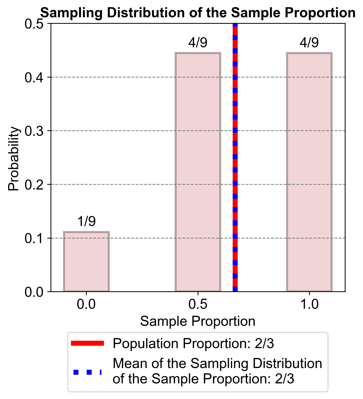
Fig. 5.56 Sampling Distribution of the Sample Proportion - This bar graph illustrates the probabilities of different sample proportions within an unspecified population. The x-axis represents the sample proportions, and the y-axis represents the probabilities. The bars show that the most likely sample proportions are 0.5 and 1.0, followed by 0.0.

Example 5.27

Consider the population {1, 2, 3, 4, 5}. Assume that samples of size \(n = 2\) are randomly selected with replacement.

• a. For the population, find the proportion of numbers greater than 3.

• b. Construct a table representing the sampling distribution of the sample proportion of numbers greater than 3. Then combine values of the sample proportion that are the same.

• c. Find the mean of the sampling distribution of the sample proportion of numbers greater than 3.

• d. Based on the preceding results, is the sample proportion an unbiased estimator of the population proportion? Why or why not?

Solution:

a. Proportion of Numbers Greater Than 3 in the Population:

\[\begin{equation*} \text{Proportion of numbers greater than 3} = \dfrac{\text{Number of numbers greater than 3}}{\text{Total numbers}} = \dfrac{2}{5} \end{equation*}\]

There are two numbers greater than 3 (4 and 5) in the population of {1, 2, 3, 4, 5}.

b. Sampling Distribution of the Sample Proportion: The possible samples of size 2 are

{(1, 1), (1, 2), (1, 3), (1, 4), (1, 5), (2, 1), (2, 2), (2, 3), (2, 4), (2, 5), (3, 1), (3, 2), (3, 3), (3, 4), (3, 5), (4, 1), (4, 2), (4, 3), (4, 4), (4, 5), (5, 1), (5, 2), (5, 3), (5, 4), (5, 5)},

which have the following proportions of numbers greater than 3:

{0, 0, 0, 1/2, 1/2, 0, 0, 0, 1/2, 1/2, 0, 0, 0, 1/2, 1/2, 1/2, 1/2, 1/2, 1, 1, 1/2, 1/2, 1/2, 1, 1}.

Sample	Sample Proportion \(\hat{p}\)	Probability
1, 1	0	1/25
1, 2	0	1/25
1, 3	0	1/25
1, 4	1/2	1/25
1, 5	1/2	1/25
2, 1	0	1/25
2, 2	0	1/25
2, 3	0	1/25
2, 4	1/2	1/25
2, 5	1/2	1/25
3, 1	0	1/25
3, 2	0	1/25
3, 3	0	1/25
3, 4	1/2	1/25
3, 5	1/2	1/25
4, 1	1/2	1/25
4, 2	1/2	1/25
4, 3	1/2	1/25
4, 4	1	1/25
4, 5	1	1/25
5, 1	1/2	1/25
5, 2	1/2	1/25
5, 3	1/2	1/25
5, 4	1	1/25
5, 5	1	1/25

Condensed Sampling Distribution of Proportion:

Sample Proportion \(\hat{p}\)	Probability
0	9/25
1/2	12/25
1	4/25

c. Mean of the Sampling Distribution of the Sample Proportion:

\[\begin{equation*} \text{Mean} = \dfrac{9 \cdot 0 + 12 \cdot \frac{1}{2} + 4 \cdot 1}{25} = \dfrac{0 + 6 + 4}{25} = \dfrac{10}{25} = \dfrac{2}{5} \end{equation*}\]

d. Unbiased Estimator: The mean of the sampling distribution of the sample proportion of numbers greater than 3 is 2/5, which is exactly equal to the population proportion of numbers greater than 3 (2/5). Therefore, the sample proportion is an unbiased estimator of the population proportion in this case.

Fig. 5.57 visually represents the distribution of sample proportions for an unspecified population. The x-axis shows the sample proportions, and the y-axis shows the probabilities of these proportions occurring.

• Sample Proportion 0.0: This bar represents the proportion of samples where no elements meet a certain condition (unspecified in this context). The probability of this proportion is approximately 9/25.

• Sample Proportion 0.5: This bar represents the proportion of samples where half of the elements meet a certain condition (unspecified in this context). The probability of this proportion is approximately 12/25.

• Sample Proportion 1.0: This bar represents the proportion of samples where all elements meet a certain condition (unspecified in this context). The probability of this proportion is approximately 4/25.

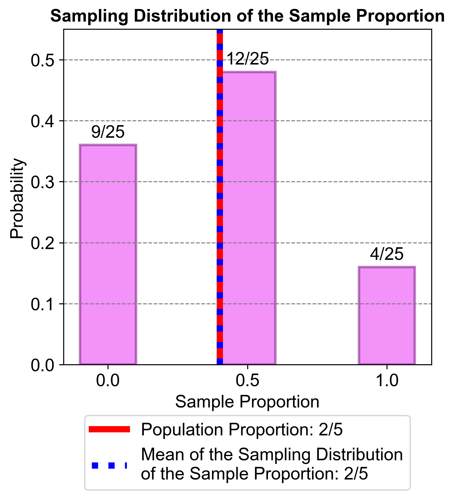
Fig. 5.57 Figure: Sampling Distribution of the Sample Proportion - This bar graph illustrates the probabilities of different sample proportions within an unspecified population. The x-axis represents the sample proportions, and the y-axis represents the probabilities. The bars show that the most likely sample proportion is 0.5, followed by 0.0 and 1.0.

Example 5.28

Consider the population {1, 2, 3, 4, 5}. Assume that samples of size \(n = 2\) are randomly selected with replacement.

• a. For the population, find the proportion of numbers less than 4.

• b. Construct a table representing the sampling distribution of the sample proportion of numbers less than 4. Then combine values of the sample proportion that are the same.

• c. Find the mean of the sampling distribution of the sample proportion of numbers less than 4.

• d. Based on the preceding results, is the sample proportion an unbiased estimator of the population proportion? Why or why not?

Solution:

a. Proportion of Numbers Less Than 4 in the Population:

\[\begin{equation*} \text{Proportion of numbers less than 4} = \dfrac{\text{Number of numbers less than 4}}{\text{Total numbers}} = \dfrac{3}{5} \end{equation*}\]

There are three numbers less than 4 (1, 2, and 3) in the population of {1, 2, 3, 4, 5}.

b. Sampling Distribution of the Sample Proportion: The possible samples of size 2 are

{(1, 1), (1, 2), (1, 3), (1, 4), (1, 5), (2, 1), (2, 2), (2, 3), (2, 4), (2, 5), (3, 1), (3, 2), (3, 3), (3, 4), (3, 5), (4, 1), (4, 2), (4, 3), (4, 4), (4, 5), (5, 1), (5, 2), (5, 3), (5, 4), (5, 5)},

which have the following proportions of numbers less than 4:

{1, 1, 1, 1/2, 1/2, 1, 1, 1, 1/2, 1/2, 1, 1, 1, 1/2, 1/2, 1/2, 1/2, 1/2, 0, 0, 1/2, 1/2, 1/2, 0, 0}.

Sample	Sample Proportion \(\hat{p}\)	Probability
1, 1	1	1/25
1, 2	1	1/25
1, 3	1	1/25
1, 4	1/2	1/25
1, 5	1/2	1/25
2, 1	1	1/25
2, 2	1	1/25
2, 3	1	1/25
2, 4	1/2	1/25
2, 5	1/2	1/25
3, 1	1	1/25
3, 2	1	1/25
3, 3	1	1/25
3, 4	1/2	1/25
3, 5	1/2	1/25
4, 1	1/2	1/25
4, 2	1/2	1/25
4, 3	1/2	1/25
4, 4	0	1/25
4, 5	0	1/25
5, 1	1/2	1/25
5, 2	1/2	1/25
5, 3	1/2	1/25
5, 4	0	1/25
5, 5	0	1/25

Condensed Sampling Distribution of Proportion:

Sample Proportion \(\hat{p}\)	Probability
0	4/25
1/2	12/25
1	9/25

c. Mean of the Sampling Distribution of the Sample Proportion:

\[\begin{equation*} \text{Mean} = \dfrac{4 \cdot 0 + 12 \cdot \frac{1}{2} + 9 \cdot 1}{25} = \dfrac{0 + 6 + 9}{25} = \dfrac{15}{25} = \dfrac{3}{5} \end{equation*}\]

d. Unbiased Estimator: The mean of the sampling distribution of the sample proportion of numbers less than 4 is 3/5, which is exactly equal to the population proportion of numbers less than 4 (3/5). Therefore, the sample proportion is an unbiased estimator of the population proportion in this case.

Fig. 5.58 visually represents the distribution of sample proportions for numbers less than 4 in the population {1, 2, 3, 4, 5}. The x-axis shows the sample proportions, and the y-axis shows the probabilities of these proportions occurring.

• Sample Proportion 0.0: This bar represents the proportion of samples where no numbers are less than 4. The probability of this proportion is approximately 4/25.

• Sample Proportion 0.5: This bar represents the proportion of samples where half of the numbers are less than 4. The probability of this proportion is approximately 12/25.

• Sample Proportion 1.0: This bar represents the proportion of samples where all numbers are less than 4. The probability of this proportion is approximately 9/25.

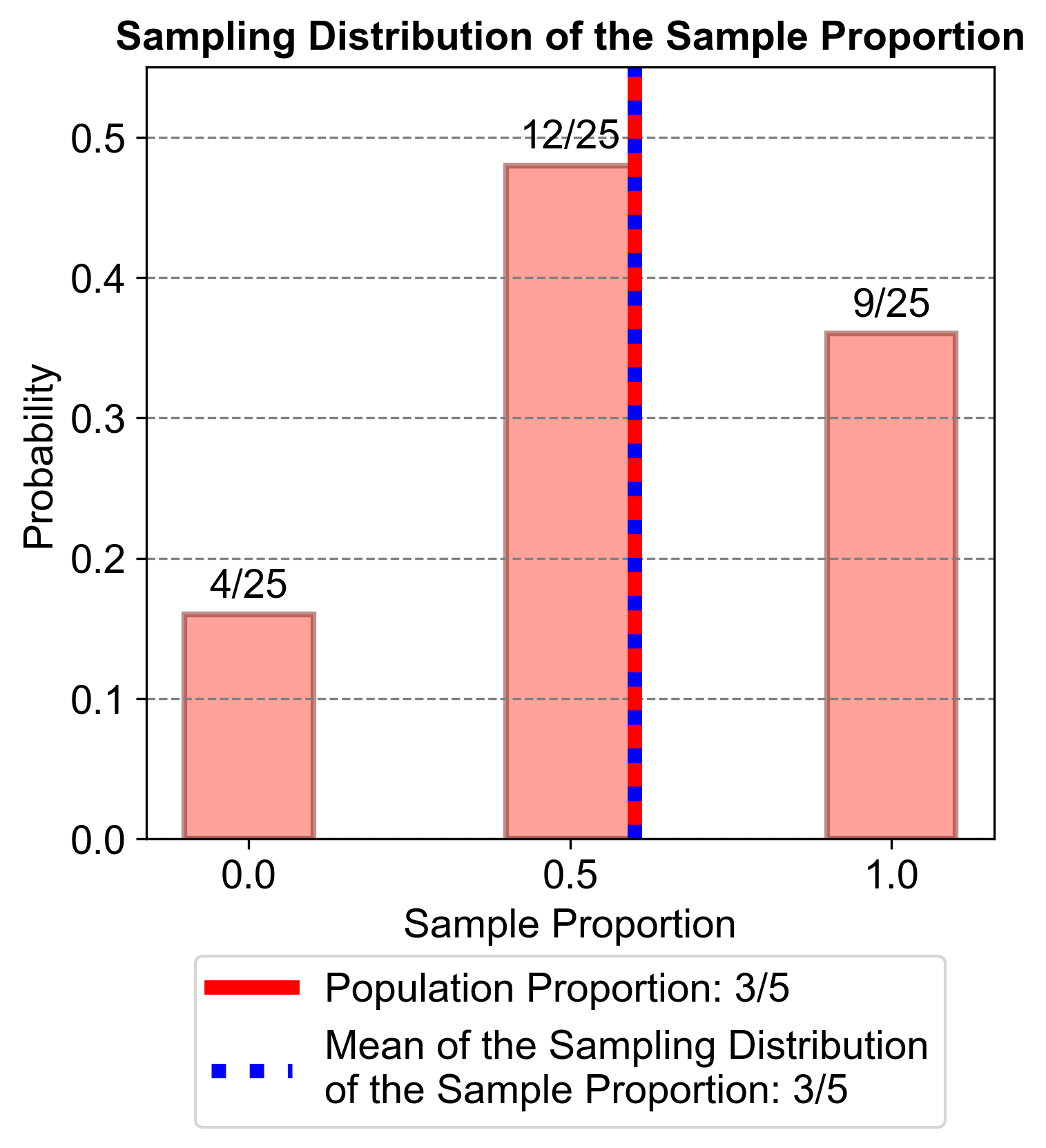
Fig. 5.58 Figure: Sampling Distribution of the Sample Proportion - This bar graph illustrates the probabilities of different sample proportions for numbers less than 4 in the population {1, 2, 3, 4, 5}. The x-axis represents the sample proportions, and the y-axis represents the probabilities. The bars show that the most likely sample proportion is 0.5, followed by 1.0 and 0.0.

Note - Key Points to Remember

• The sampling distribution of the sample proportion becomes approximately normal as the sample size increases.

• The mean of the sampling distribution of the sample proportion is equal to the population proportion.

• The standard deviation of the sampling distribution of the sample proportion decreases as the sample size increases.

5.6.4. Sampling Distribution of the Sample Mean

Understanding the sampling distribution of the sample mean is fundamental in statistics, as it forms the basis for many inferential techniques.

Definition - Sampling Distribution of the Sample Mean

The sampling distribution of the sample mean refers to the distribution of all possible sample means (denoted as \(\bar{x}\)) that could be obtained from samples of a fixed size \(n\) drawn from the same population. This distribution is typically illustrated as a probability distribution, which can be represented by a probability histogram, a formula, or a table.

5.6.4.1. Behavior of Sample Means

The characteristics of the sampling distribution of the sample mean are crucial for making inferences about the population mean.

Behavior of Sample Means

1. Normal Distribution: The distribution of sample means tends to approximate a normal distribution, particularly as the sample size increases. This phenomenon is a consequence of the Central Limit Theorem, which states that, regardless of the population distribution, the sampling distribution of the sample mean will be approximately normal for sufficiently large sample sizes.

2. Targeting Population Mean: The sample means converge around the population mean. This implies that the mean of the sampling distribution of the sample means is equal to the population mean (\(\mu\)). Therefore, the expected value of the sample mean is the population mean.

5.6.4.2. Sampling Error

While sample means provide valuable estimates of the population mean, it is important to consider the inherent variability in these estimates.

Definition - Sampling Error

Sampling error refers to the discrepancy between the sample mean and the true population mean, which arises due to the fact that only a subset of the population is used to estimate the population parameter.

5.6.4.3. Impact of Sample Size on Sampling Error

The size of the sample plays a critical role in the accuracy of the sample mean as an estimate of the population mean.

Note - Sample Size and Sampling Error

The larger the sample size, the smaller the sampling error tends to be. As the sample size increases, the sample mean becomes a more reliable estimate of the population mean (\(\mu\)), thereby reducing the variability of the sample means around the population mean.

Example 5.29

Suppose we have a small population of students with the following heights (in cm): {150, 160, 170}. We want to study the sampling distribution of the sample mean by randomly selecting two heights with replacement from this population.

1. What is the population mean (\(\mu\))?

2. What are the possible samples of size 2?

3. What are the sample means and their probabilities?

4. What is the condensed sampling distribution of the sample mean?

5. What is the mean of the sample means, and does it target the population mean?

Solution:

1. Population Mean:

   \[\begin{equation*} \mu = \dfrac{150 + 160 + 170}{3} = 160 \end{equation*}\]

2. Possible Samples of Size 2:

{(150, 150), (150, 160), (150, 170), (160, 150), (160, 160), (160, 170), (170, 150), (170, 160), (170, 170)}

3. Sample Means and Probabilities:

Sample	Sample Mean \(\bar{x}\)	Probability
150, 150	150	1/9
150, 160	155	1/9
150, 170	160	1/9
160, 150	155	1/9
160, 160	160	1/9
160, 170	165	1/9
170, 150	160	1/9
170, 160	165	1/9
170, 170	170	1/9

4. Condensed Sampling Distribution of Mean:

Sample Mean \(\bar{x}\)	Probability
150	1/9
155	2/9
160	3/9
165	2/9
170	1/9

5. Mean of the Sample Means:

   \[\begin{equation*} \mu_{\bar{x}} = 150 \cdot \frac{1}{9} + 155 \cdot \frac{2}{9} + 160 \cdot \frac{3}{9} + 165 \cdot \frac{2}{9} + 170 \cdot \frac{1}{9} = 160 \end{equation*}\]

Since the mean of the sample means (160) is equal to the mean of the population (160), we conclude that the values of the sample mean do target the value of the population mean.

Fig. 5.59 visually represents the condensed sampling distribution mentioned in part four of the provided context. It shows how different samples can have different probabilities and that most samples are centered around the population mean (160), supporting the conclusion that sample means target the population mean.

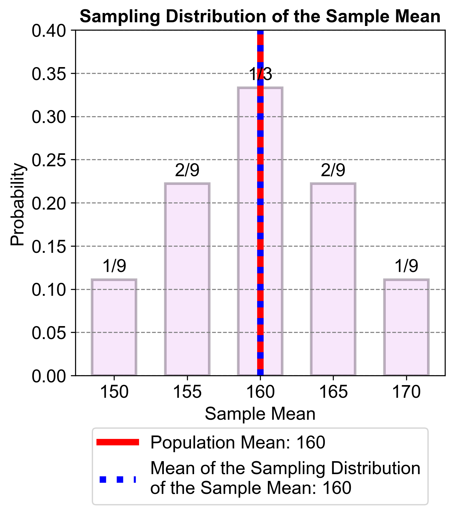
Fig. 5.59 The figure illustrates the condensed sampling distribution of the sample mean for a small population of students with heights {150, 160, 170} cm. The sampling distribution is derived by randomly selecting two heights with replacement from this population. The probabilities of the sample means are shown, demonstrating that the sample means target the population mean (160 cm).

Example 5.30

Suppose we have a small population of students with the following test scores: {70, 80, 90}. We want to study the sampling distribution of the sample mean by randomly selecting two scores with replacement from this population.

• a. What is the population mean (\(\mu\))?

• b. What are the possible samples of size 2?

• c. What are the sample means and their probabilities?

• d. What is the condensed sampling distribution of the sample mean?

• e. What is the mean of the sample means, and does it target the population mean?

Solution:

1. Population Mean:

   \[\begin{equation*} \mu = \dfrac{70 + 80 + 90}{3} = 80 \end{equation*}\]

2. Possible Samples of Size 2:

{(70, 70), (70, 80), (70, 90), (80, 70), (80, 80), (80, 90), (90, 70), (90, 80), (90, 90)}

3. Sample Means and Probabilities:

Sample	Sample Mean \(\bar{x}\)	Probability
70, 70	70	1/9
70, 80	75	1/9
70, 90	80	1/9
80, 70	75	1/9
80, 80	80	1/9
80, 90	85	1/9
90, 70	80	1/9
90, 80	85	1/9
90, 90	90	1/9

4. Condensed Sampling Distribution of Mean:

Sample Mean \(\bar{x}\)	Probability
70	1/9
75	2/9
80	3/9
85	2/9
90	1/9

5. Mean of the Sample Means:

   \[\begin{equation*} \mu_{\bar{x}} = 70 \cdot \frac{1}{9} + 75 \cdot \frac{2}{9} + 80 \cdot \frac{3}{9} + 85 \cdot \frac{2}{9} + 90 \cdot \frac{1}{9} = 80 \end{equation*}\]

Since the mean of the sample means (80) is equal to the mean of the population (80), we conclude that the values of the sample mean do target the value of the population mean.

Fig. 5.60 visually represents the condensed sampling distribution mentioned in part four of the provided context. It shows how different samples can have different probabilities and that most samples are centered around the population mean (80), supporting the conclusion that sample means target the population mean.

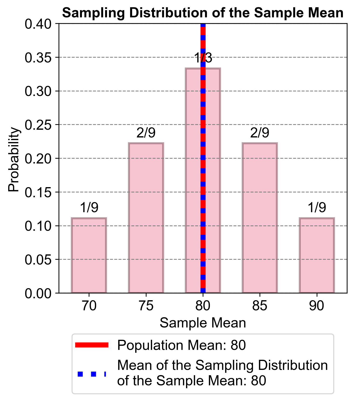
Fig. 5.60 The figure illustrates the condensed sampling distribution of the sample mean for a small population of students with test scores {70, 80, 90}. The sampling distribution is derived by randomly selecting two scores with replacement from this population. The probabilities of the sample means are shown, demonstrating that the sample means target the population mean (80).

5.6.5. Sampling Distribution of the Sample Variance

The sampling distribution of the sample variance is essential in understanding how variance estimates behave across different samples taken from the same population.

Definition - Sampling Distribution of the Sample Variance

The sampling distribution of the sample variance refers to the distribution of sample variances (denoted as \(s^2\)) computed from all possible samples of a fixed size \(n\) drawn from the same population. This distribution is often represented as a probability distribution, which can be visualized through a table, probability histogram, or formula.

5.6.5.1. Behavior of Sample Variances

Understanding the characteristics of the sampling distribution of the sample variance is crucial for making inferences about the population variance.

Behavior of Sample Variances

1. Skewed Distribution: The distribution of sample variances tends to be skewed to the right. This skewness implies that while most sample variances are relatively small, there are occasional large values, leading to a longer tail on the right side of the distribution.

2. Targeting Population Variance: The sample variances are centered around the population variance. This means that the mean of the sampling distribution of the sample variances is equal to the population variance (\(\sigma^2\)). In statistical terms, the expected value of the sample variance is the population variance.

5.6.5.2. Importance of the Sampling Distribution of the Sample Variance

The sampling distribution of the sample variance provides insight into the variability of sample variances when multiple samples are drawn from the same population.

By analyzing this distribution, one can make informed inferences about the population variance. The right skewness indicates that although most sample variances are close to the population variance, some samples may produce significantly larger variances, highlighting the variability in variance estimates across samples.

Example 5.31

Suppose we have a small population of students with the following test scores: {60, 70, 80}. We want to study the sampling distribution of the sample variance by randomly selecting two scores with replacement from this population.

• a. What is the population variance (\(\sigma^2\))?

• b. What are the possible samples of size 2?

• c. What are the sample variances and their probabilities?

• d. What is the condensed sampling distribution of the sample variance?

• e. What is the mean of the sample variances, and does it target the population variance?

Solution:

1. Population Variance:

   \[\begin{equation*} \sigma^2 = \dfrac{(60-70)^2 + (70-70)^2 + (80-70)^2}{3} = \dfrac{100 + 0 + 100}{3} = \dfrac{200}{3} \approx 66.67 \end{equation*}\]

2. Possible Samples of Size 2:

{(60, 60), (60, 70), (60, 80), (70, 60), (70, 70), (70, 80), (80, 60), (80, 70), (80, 80)}

3. Sample Variances and Probabilities:

Sample	Sample Variance \(s^2\)	Probability
60, 60	0	1/9
60, 70	25	1/9
60, 80	100	1/9
70, 60	25	1/9
70, 70	0	1/9
70, 80	25	1/9
80, 60	100	1/9
80, 70	25	1/9
80, 80	0	1/9

4. Condensed Sampling Distribution of Variance:

Sample Variance \(s^2\)	Probability
0	3/9
25	4/9
100	2/9

5. Mean of the Sample Variances:

   \[\begin{equation*} \text{Mean} = \dfrac{3 \cdot 0 + 4 \cdot 25 + 2 \cdot 100}{9} = \dfrac{0 + 100 + 200}{9} = \dfrac{300}{9} \approx 33.33 \end{equation*}\]

Since the mean of the sample variances (33.33) is not equal to the population variance (66.67), we conclude that the sample variances do not target the value of the population variance.

Fig. 5.61 visually represents the condensed sampling distribution mentioned in part four of the provided context. It shows how different samples can have different probabilities and that the sample variances do not target the population variance (66.67).

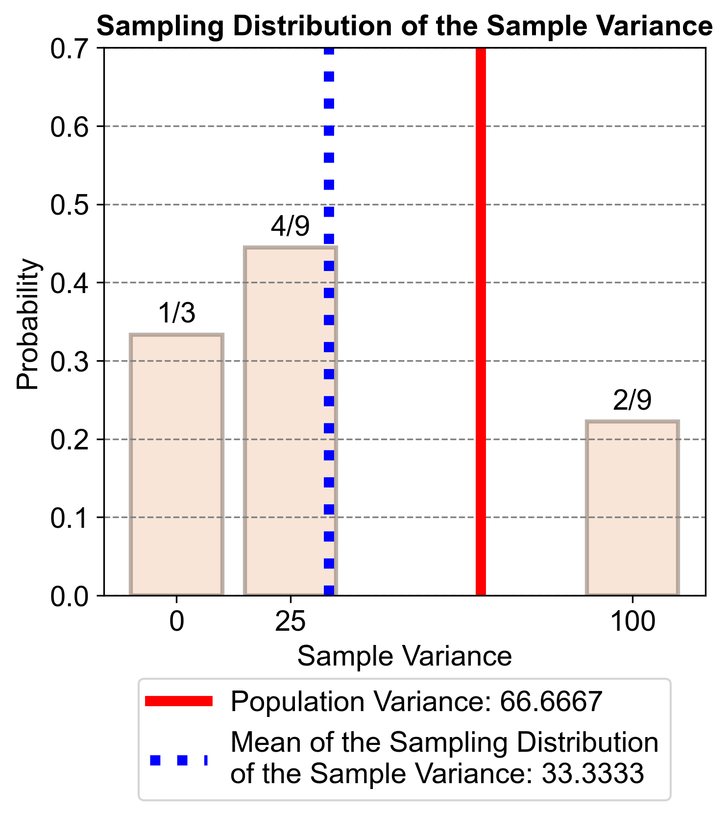
Fig. 5.61 The figure illustrates the condensed sampling distribution of the sample variance for a small population of students with test scores {60, 70, 80}. The sampling distribution is derived by randomly selecting two scores with replacement from this population. The probabilities of the sample variances are shown, demonstrating that the sample variances do not target the population variance (66.67).

Example 5.32

Suppose we have a small population of plants with the following heights (in cm): {10, 15, 20}. We want to study the sampling distribution of the sample variance by randomly selecting two heights with replacement from this population.

• a. What is the population variance (\(\sigma^2\))?

• b. What are the possible samples of size 2?

• c. What are the sample variances and their probabilities?

• d. What is the condensed sampling distribution of the sample variance?

• e. What is the mean of the sample variances, and does it target the population variance?

Solution:

1. Population Variance:

   \[\begin{equation*} \sigma^2 = \dfrac{(10-15)^2 + (15-15)^2 + (20-15)^2}{3} = \dfrac{25 + 0 + 25}{3} = \dfrac{50}{3} \approx 16.67 \end{equation*}\]

2. Possible Samples of Size 2:

{(10, 10), (10, 15), (10, 20), (15, 10), (15, 15), (15, 20), (20, 10), (20, 15), (20, 20)}

3. Sample Variances and Probabilities:

Sample	Sample Variance \(s^2\)	Probability
10, 10	0	1/9
10, 15	6.25	1/9
10, 20	25	1/9
15, 10	6.25	1/9
15, 15	0	1/9
15, 20	6.25	1/9
20, 10	25	1/9
20, 15	6.25	1/9
20, 20	0	1/9

4. Condensed Sampling Distribution of Variance:

Sample Variance \(s^2\)	Probability
0	3/9
6.25	4/9
25	2/9

5. Mean of the Sample Variances:

   \[\begin{equation*} \text{Mean} = \dfrac{3 \cdot 0 + 4 \cdot 6.25 + 2 \cdot 25}{9} = \dfrac{0 + 25 + 50}{9} = \dfrac{75}{9} \approx 8.33 \end{equation*}\]

Fig. 5.62 visually represents the condensed sampling distribution mentioned in part four of the provided context. It shows how different samples can have different probabilities and that the sample variances do not target the population variance (16.67).

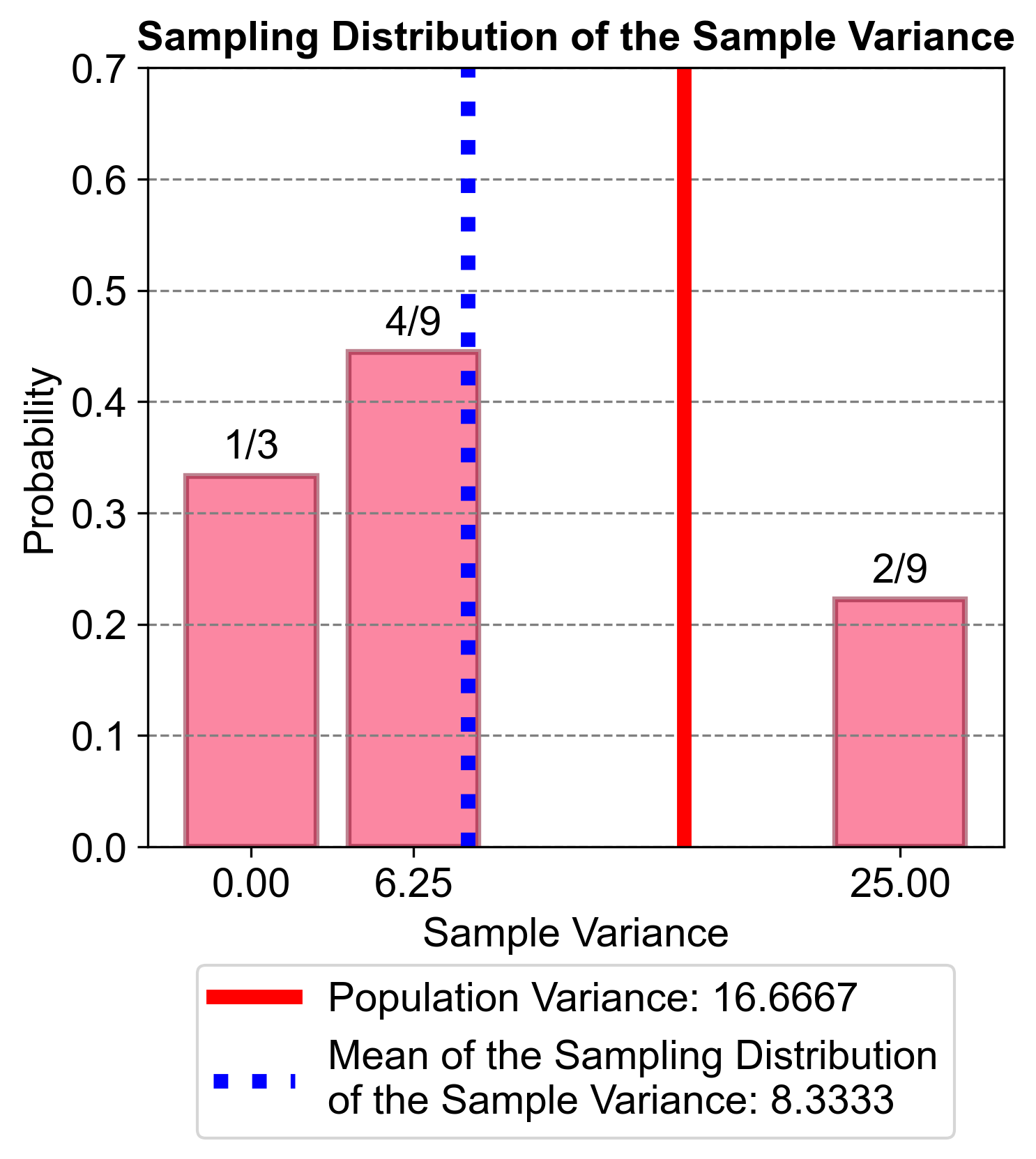
Fig. 5.62 The figure illustrates the condensed sampling distribution of the sample variance for a small population of plants with heights {10, 15, 20} cm. The sampling distribution is derived by randomly selecting two heights with replacement from this population. The probabilities of the sample variances are shown, demonstrating that the sample variances do not target the population variance (16.67).