6.3. Understanding the t-Distribution

In statistical analysis, degrees of freedom (df) represent the number of values that can vary independently, given certain constraints. In practice, they measure the amount of information available for accurately estimating a population parameter.

6.3.1. Degrees of Freedom in t-Distributions

The t-distribution is a probability distribution used for small sample sizes and unknown population variances. While it resembles the normal distribution, the t-distribution has heavier tails, accommodating the increased uncertainty in small samples. Its shape changes based on sample size, determined by degrees of freedom.

For the t-distribution, degrees of freedom are calculated as \(df = n - 1\), where n is the sample size. This reflects the number of values in the sample that are free to vary.

Note

Degrees of freedom are conceptually similar to having ‘\(n\)’ puzzle pieces with one piece predetermined. The remaining ‘\(n - 1\)’ pieces represent the degrees of freedom, which limits the flexibility in arranging the remaining data values.

6.3.2. Studentized Version of the Sample Mean

To make comparisons with theoretical distributions like the t-distribution, sample means are often standardized, a process called “studentizing.” This standardization results in the Student’s t-distribution.

The studentized form for a sample mean \(\overline{x}\) is given by:

(6.4)\[\begin{equation} t = \frac{\overline{x} - \mu}{\frac{s}{\sqrt{n}}} \end{equation}\]

where:

• ‘\(t\)’ is the test statistic following a t-distribution with \(df = n - 1\),

• ‘\(\overline{x}\)’ is the sample mean,

• ‘\(\mu\)’ is the population mean (or hypothesized mean in inferential testing),

• ‘\(s\)’ is the sample standard deviation,

• ‘\(n\)’ is the sample size.

Note

The studentized sample mean is essential when the population standard deviation is unknown, which is commonly the case in real-world analyses.

6.3.3. Visualizing the t-Curve

The t-distribution is represented by a symmetric, bell-shaped curve known as the t-curve. Each t-curve is distinctively defined by its degrees of freedom, but all t-curves share the symmetry and general shape of the standard normal distribution.

A prominent feature of t-curves is their heavier tails relative to the normal distribution, reflecting a higher probability of observing values far from the mean. This characteristic accommodates the increased uncertainty in small samples. As the degrees of freedom increase, the t-curve gradually approaches the shape of the standard normal curve, becoming nearly identical at higher values of degrees of freedom.

Fig. 6.16 illustrates a comparison between t-distributions with various degrees of freedom (df) and the standard normal distribution. The horizontal axis represents t-values ranging from -4 to 4, while the vertical axis displays the probability density. The graph shows five curves: the standard normal distribution (depicted by a dashed line) and t-distributions with df = 1, 5, 10, and 20.

This visual comparison highlights how t-distributions with higher degrees of freedom more closely resemble the standard normal distribution. Conversely, t-distributions with lower degrees of freedom show more pronounced heavy tails, indicating greater variability in the data. The convergence of the t-distribution towards the normal distribution as sample size (and degrees of freedom) increases is fundamental in statistical inference and hypothesis testing.

Understanding the relationship between sample size, degrees of freedom, and distribution shape is essential for accurately interpreting statistical analyses, particularly with small sample sizes or unknown population parameters. This concept supports numerous statistical methods and informs data-based decision-making.

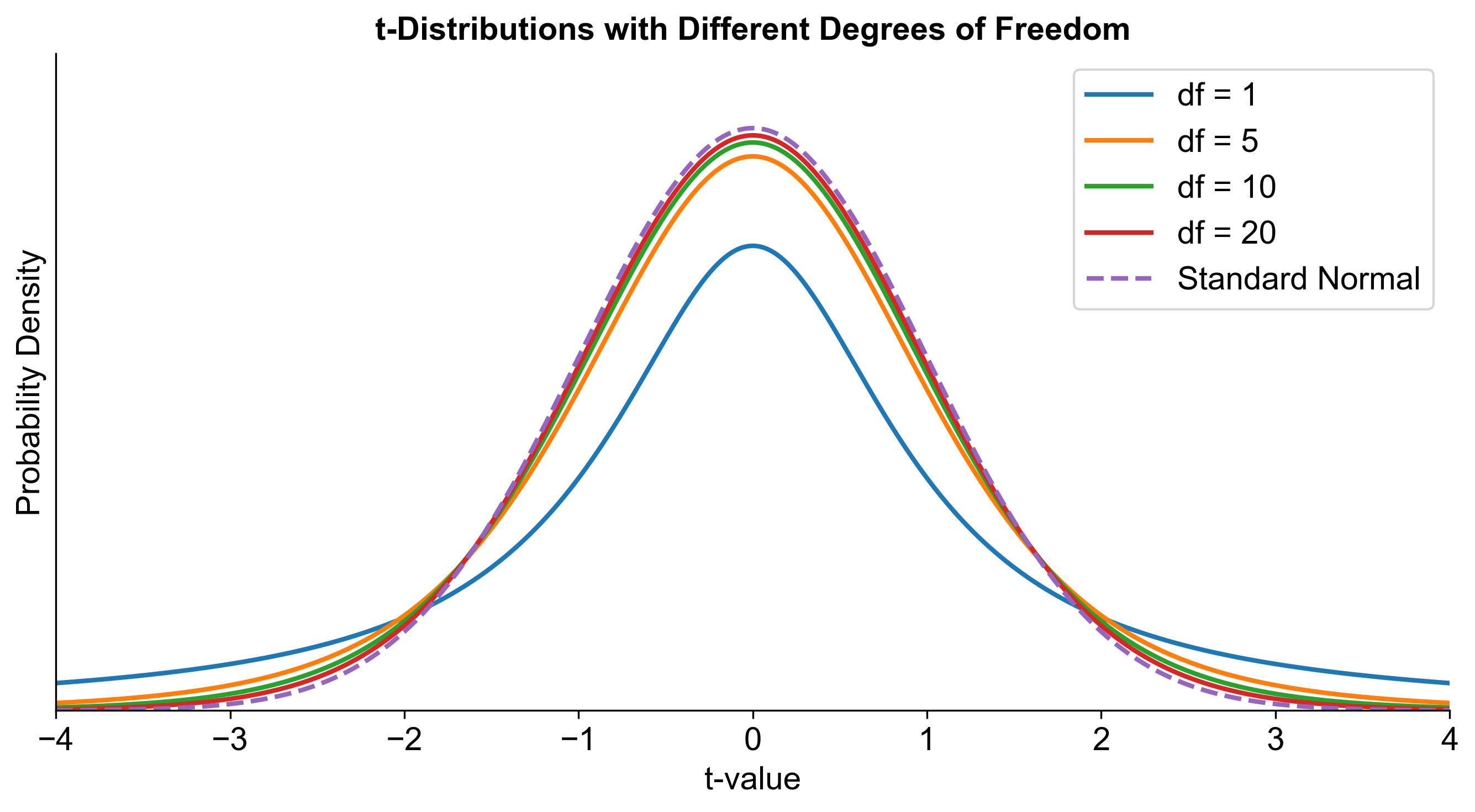
Fig. 6.16 Comparison of t-Distributions with Varying Degrees of Freedom to Standard Normal Distribution

Note

It’s important to visualize the t-curve not just as a static image but as a dynamic shape that changes with the degrees of freedom. This helps in understanding the impact of sample size on the distribution.

Characteristics of the Student’s t-Distribution

1. The graph of the Student’s t-distribution shares similarities with the standard normal curve.

2. The mean of the Student’s t-distribution is zero, and the distribution exhibits symmetry around zero.

3. Compared to the standard normal distribution, the Student’s t-distribution has more probability in its tails. This is because the t-distribution has a larger spread than the standard normal distribution. As a result, the graph of the Student’s t-distribution will appear thicker in the tails and shorter in the center than the graph of the standard normal distribution.

4. The precise form of the Student’s t-distribution is determined by its degrees of freedom. As the degrees of freedom increase, the graph of the Student’s t-distribution progressively resembles the graph of the standard normal distribution.

5. We assume that the underlying population of individual observations follows a normal distribution with unknown population mean (\(\mu\)) and unknown population standard deviation (\(\sigma\)). Typically, the size of the underlying population is not a crucial factor unless it is exceptionally small. When the population distribution exhibits a bell-shaped (normal) pattern, this assumption is satisfied and requires no further discussion. Random sampling is also assumed, but it is a distinct assumption and should not be confused with the assumption of normality.

6.3.4. Determining t-Value

To determine the t-value \(t_{0.05, 10}\) corresponding to an area of 0.05 (5% probability) in the right tail of the t-distribution with degrees of freedom (df) equal to 10, we consult a t-distribution table. The t-distribution table provides critical values for different degrees of freedom and significance levels (\(\alpha\)).

Degrees of Freedom (df) represent the number of independent values in a dataset that can vary freely. In the t-distribution table, df is listed vertically on the left side.

Significance Level (\(\alpha\)) denotes the probability of rejecting the null hypothesis when it is true. Common significance levels such as 0.10, 0.05, 0.025, etc., are listed horizontally at the top of the table.

The Critical t-value (\(t_{\alpha, df}\)) is the value from the t-distribution corresponding to the chosen significance level and degrees of freedom. For instance, \(t_{0.05, 10}\) is the critical value for a 5% significance level with 10 degrees of freedom.

To find \(t_{0.05, 10}\), locate the row for df=10 and the column for \(\alpha=0.05\) in the t-distribution table. The intersection provides the critical t-value, which is 1.812. This implies that only 5% of the t-distribution lies beyond the t-value of 1.812 for a one-tailed t-test with df=10. If your computed t-statistic exceeds 1.812, you would reject the null hypothesis at the 5% significance level.

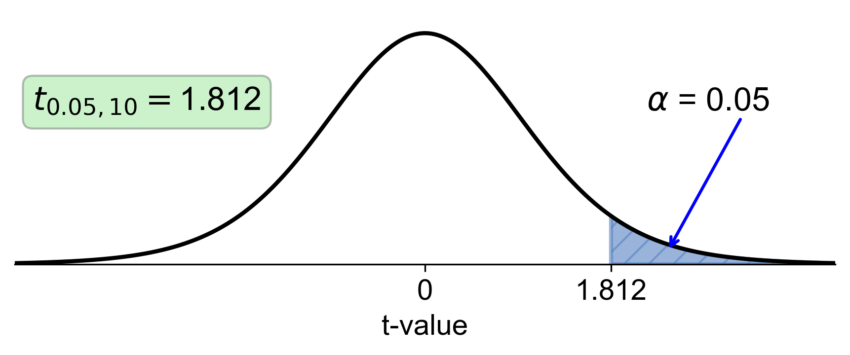
Fig. 6.17 Visualization of t-distribution with 10 degrees of freedom and right-tail area of 0.05

We could also consider finding the t-value \(t_{0.1, 20}\) corresponding to an area of 0.1 (10% probability) in the right tail of the t-distribution with degrees of freedom (df) equal to 20. This involves referencing a t-distribution table to identify the critical t-value.

Degrees of Freedom (df): This represents the number of independent values in a dataset that are free to vary. In the t-distribution table, df is listed vertically on the left side.

Significance Level (\(\alpha\)): This is the probability of rejecting the null hypothesis when it is actually true. Here, \(\alpha = 0.1\) corresponds to a 10% significance level, which is listed horizontally at the top of the table.

The Critical t-value (\(t_{\alpha, df}\)) is the value from the t-distribution that corresponds to the chosen significance level and degrees of freedom. For \(t_{0.1, 20}\), this is the critical value for a 10% significance level with 20 degrees of freedom.

In our example, \(t_{0.1, 20}\) is given as 1.325. This means that for a one-tailed t-test with df = 20, only 10% of the t-distribution lies beyond the t-value of 1.325. If your computed t-statistic exceeds 1.325, you would reject the null hypothesis at the 10% significance level.

To find \(t_{0.1, 20}\) in a t-distribution table, locate the row for df = 20 and the column for \(\alpha = 0.1\). The intersection provides the critical t-value, which is 1.325 in this case.

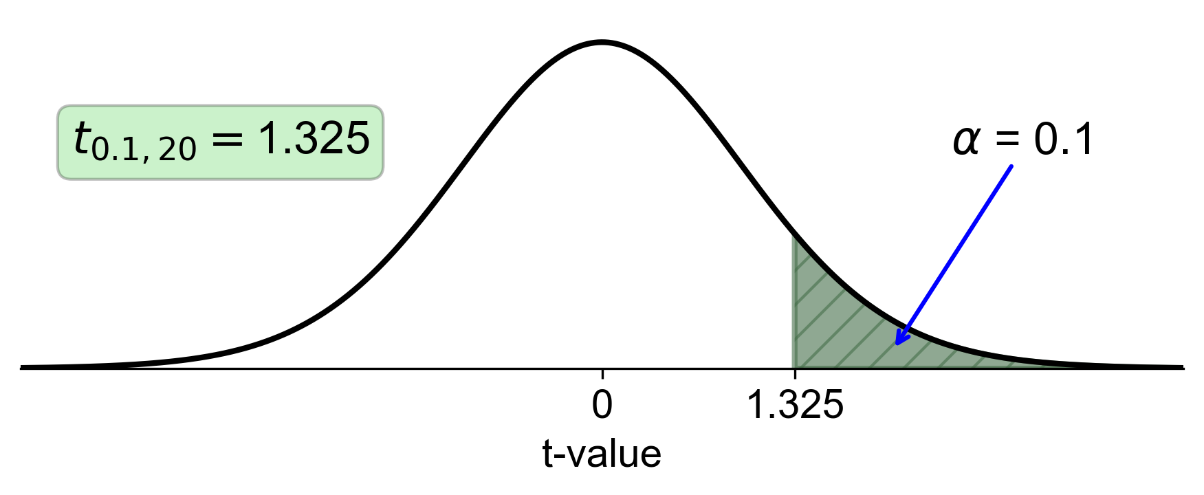
Fig. 6.18 Visualization of t-distribution with 20 degrees of freedom and right-tail area of 0.1

6.3.5. t-distribution Table

To use the provided t-distribution table here, where the top row indicates different significance levels (\(\alpha\)) corresponding to the right-hand side area of the t-distribution, and the left column lists degrees of freedom (df), follow these steps:

1. Identify Degrees of Freedom (df): Determine the degrees of freedom for your t-test. For example, if df = 20, locate the row labeled “20”.

2. Select the Significance Level (\(\alpha\)): Choose the significance level for your hypothesis test. This is typically predetermined based on the desired level of confidence. For instance, if \(\alpha = 0.1\), find the column labeled “0.1”.

3. Locate the Intersection: The intersection of the row for df = 20 and the column for \(\alpha = 0.1\) gives you the critical t-value (\(t_{0.1, 20}\)) from the t-distribution table.

4. Read the Critical t-value: In the provided table, the critical t-value for df = 20 and \(\alpha = 0.1\) is 1.325.

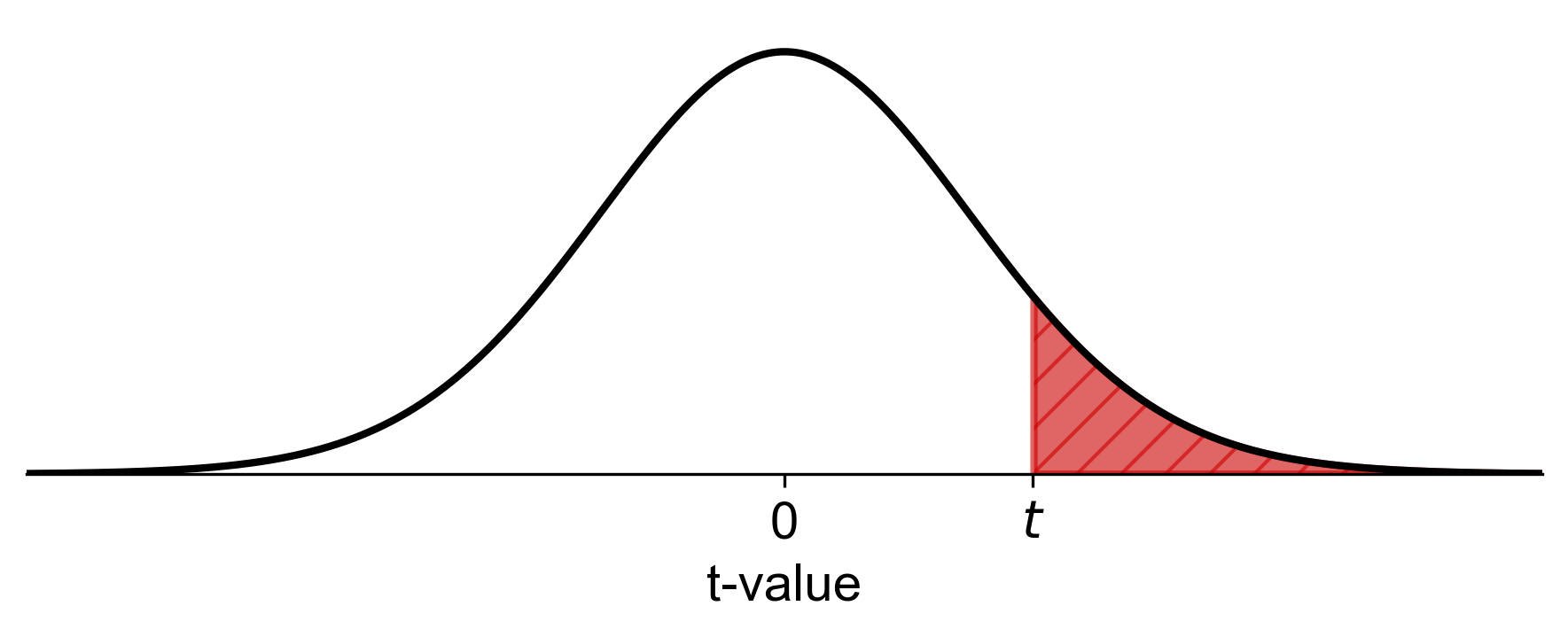
Fig. 6.19 Visualization of t-distribution with right-tail area

	0.1	0.05	0.025	0.01	0.005	0.001
df
Loading ITables v2.2.3 from the init_notebook_mode cell... (need help?)

Example 6.19 (Finding a t-Value Using the t-Distribution Table)

For parts (a)-(d), find the critical t-value.

• a): Degrees of Freedom (df) = 5 and Right-Hand Side Area = 0.01

• b): Degrees of Freedom (df) = 15 and Right-Hand Side Area = 0.025

• c): Degrees of Freedom (df) = 24 and Right-Hand Side Area = 0.001

• d): Degrees of Freedom (df) = 31 and Right-Hand Side Area = 0.05

Solution: To find the critical t-values, we use the provided t-distribution table with the specified degrees of freedom (df) and areas.

Part a:

• Degrees of Freedom (df): 5

• Right-Hand Side Area (α): 0.01

• Critical t-value: 3.365 (from the intersection of df = 5 and \(\alpha\) = 0.01)

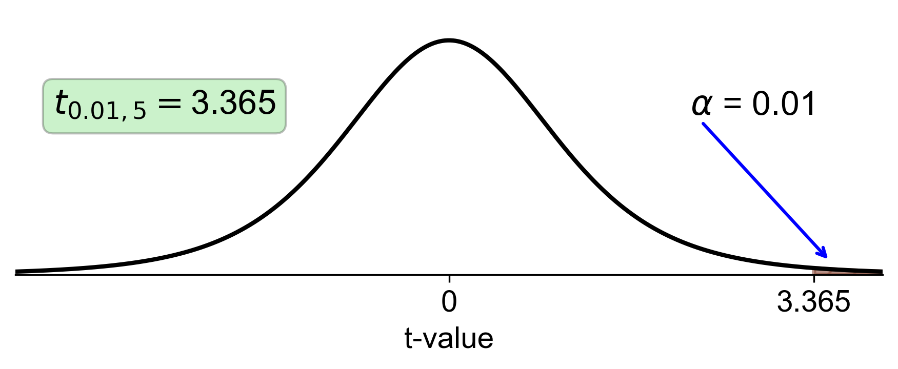
Fig. 6.20 t-distribution with 5 degrees of freedom and right-tail area of 0.01

Fig. 6.20 shows the t-distribution with 5 degrees of freedom. The shaded area represents the right-tail area of 0.01, and the vertical line indicates the critical t-value of 3.365.

Part b:

• Degrees of Freedom (df): 15

• Right-Hand Side Area (α): 0.025

• Critical t-value: 2.131 (from the intersection of df = 15 and \(\alpha\) = 0.025)

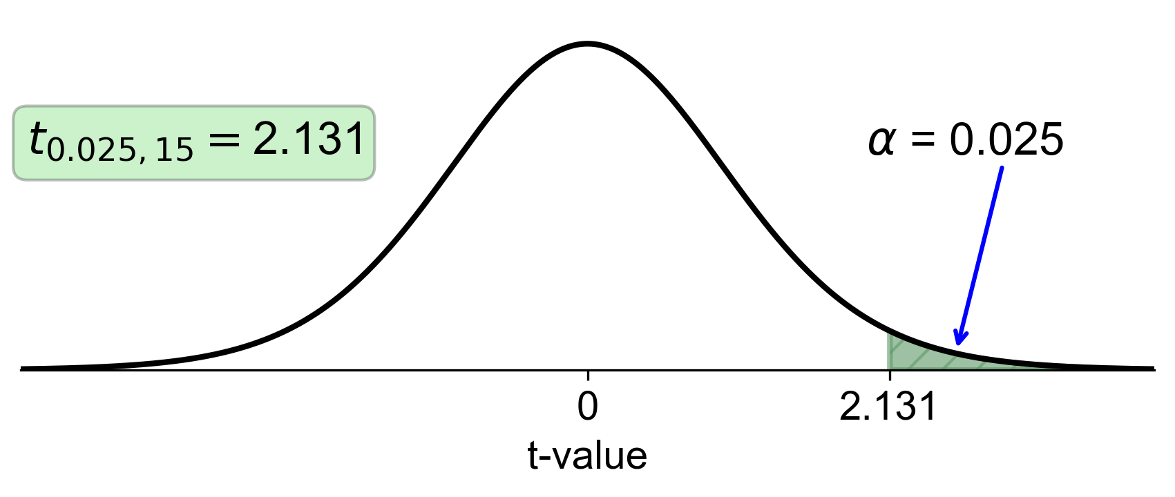
Fig. 6.21 t-distribution with 15 degrees of freedom and right-tail area of 0.025

Fig. 6.21 illustrates the t-distribution with 15 degrees of freedom. The shaded area represents the right-tail area of 0.025, and the vertical line shows the critical t-value of 2.131.

Part c:

• Degrees of Freedom (df): 24

• Right-Hand Side Area (α): 0.001

• Critical t-value: 3.467 (from the intersection of df = 24 and \(\alpha\) = 0.001)

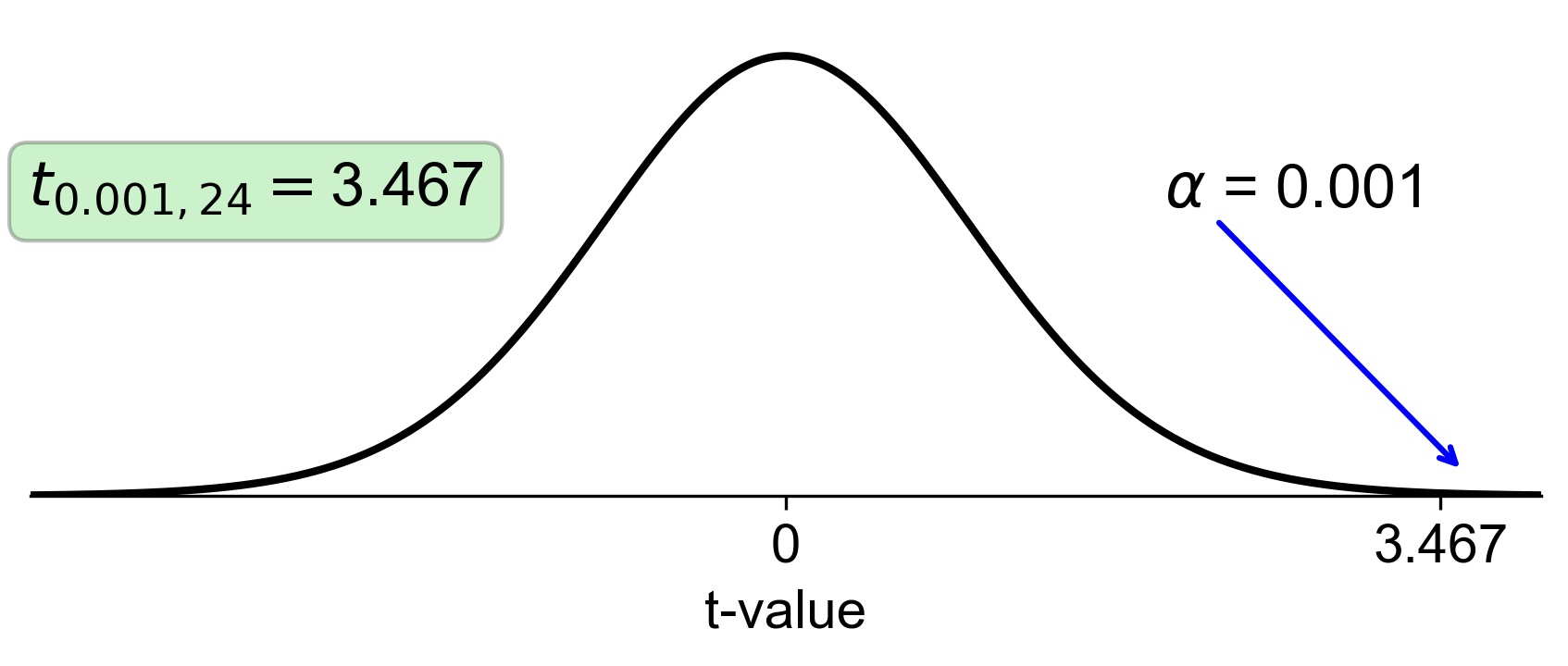
Fig. 6.22 t-distribution with 24 degrees of freedom and right-tail area of 0.001

Fig. 6.22 displays the t-distribution with 24 degrees of freedom. The shaded area represents the right-tail area of 0.001, and the vertical line indicates the critical t-value of 3.467.

Part d:

• Degrees of Freedom (df): 31

• Right-Hand Side Area (α): 0.05

• Critical t-value: 1.696 (from the intersection of df = 31 and \(\alpha\) = 0.05)

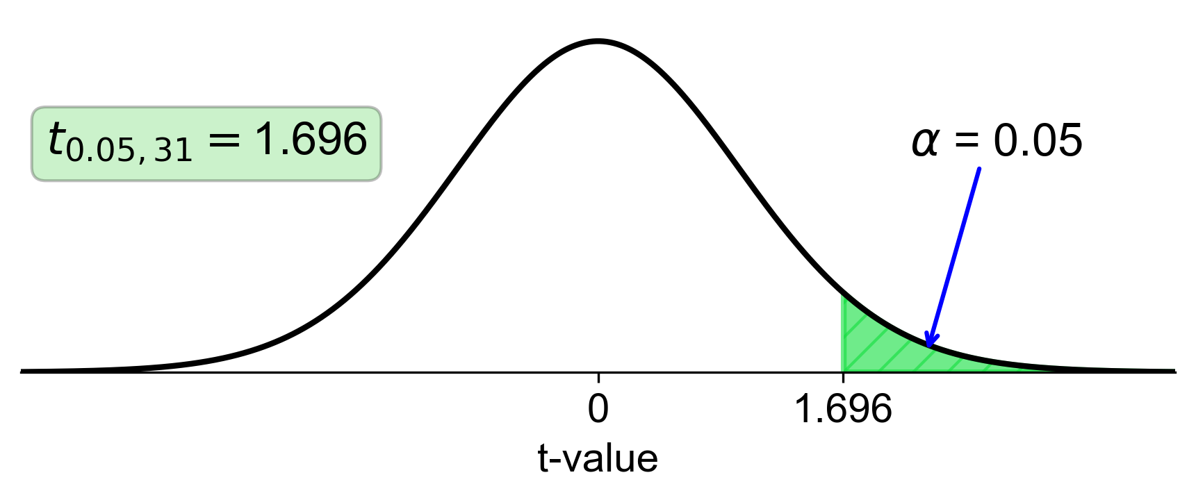
Fig. 6.23 t-distribution with 31 degrees of freedom and right-tail area of 0.05

Fig. 6.23 shows the t-distribution with 31 degrees of freedom. The shaded area represents the right-tail area of 0.05, and the vertical line indicates the critical t-value of 1.696.