4.4. Poisson Distribution#
Definition - Poisson Probability Distribution
The Poisson probability distribution is a discrete statistical distribution that estimates the probability of a specified number of events happening within a predetermined interval. This interval could be defined in various dimensions such as time, distance, area, volume, or any other continuous measurement. The random variable “\(X\)” signifies the number of events that are expected to occur during this interval.
Key Properties:
Independent Events: The events are considered to be independent within the interval. This independence implies that the occurrence of one event does not affect the chances of another event taking place at the same or different point within the interval.
Constant Rate: The average rate of occurrence, symbolized by \(\lambda\) (lambda), is consistent throughout the interval. It represents the expected average number of events per unit of the interval.
Mathematical Representation:
The probability of exactly “x” events occurring is captured by the Poisson formula:
where:
\(e \approx 2.71828\) is Euler’s number, serving as the base for natural logarithms.
\(\lambda\) is the average number of events anticipated to happen within the interval.
\(x!\) is the factorial of “\(x\)”, which is the multiplication of all positive integers up to “x”.
Parameters:
Mean (\(\lambda\)): The mean represents the average count of events within the interval.
Variance (\(\lambda\)): The variance is also \(\lambda\), indicating that the mean and variance of the Poisson distribution are identical.
Standard Deviation (\(\sigma\)): The standard deviation is the square root of the variance, calculated as \(\sigma = \sqrt{\lambda}\).
Notation:
The notation \(X \sim \text{Pois}(\lambda)\) (or \(X \sim \text{Poisson}(\lambda)\)) denotes that the random variable “X” follows the Poisson distribution with a mean rate of \(\lambda\). This is interpreted as “X is a random variable described by a Poisson distribution with parameter \(\lambda\)”.
Applications:
The Poisson distribution is especially useful in situations where events transpire randomly and independently across a continuum. It is frequently used to model occurrences such as the number of calls a call center receives, customer arrivals at a retail store, or the decay of radioactive particles.
Limitations:
Although the Poisson distribution is broadly applicable, it is predicated on the assumption that events transpire at a uniform rate and independently from one another. In practical scenarios where these conditions are not satisfied, alternative statistical models might be more fitting.
Example 4.27
A botanical study on the distribution of a particular wildflower species in a meadow found that the average number of these flowers per square meter is 5.0. Given this information:
a. Calculate the probability of finding no wildflowers in a randomly selected 1 \(m^2\) area.
b. Determine the probability of encountering at least one wildflower in a 1 \(m^2\) plot.
c. Compute the probability of observing at most two wildflowers in a 1 \(m^2\) section.
Solution: Let \(X\) represent the number of wildflowers in a 1 \(m^2\) area. We can model this scenario using a Poisson distribution because:
We’re dealing with rare events (wildflowers) in a continuous space (the meadow).
The events occur independently of each other.
The average rate of occurrence (\(\lambda\)) is known and constant.
The Poisson distribution has a probability mass function:
where \(\lambda\) is the average rate of occurrence (in this case, 5.0 wildflowers per square meter) and \(k\) is the number of occurrences we’re interested in.
a. To find the probability of no wildflowers in a 1 \(m^2\) area:
We use \(k = 0\) in the Poisson probability mass function:
This means there’s about a 0.67% chance of finding no wildflowers in a randomly selected 1 \(m^2\) area.
b. For the probability of encountering at least one wildflower:
We can use the complement rule. The probability of at least one wildflower is the opposite of having no wildflowers:
This indicates a very high probability (about 99.33%) of finding at least one wildflower in a 1 \(m^2\) plot.
c. To compute the probability of observing at most two wildflowers:
We need to sum the probabilities of having 0, 1, and 2 wildflowers:
Interpretation:
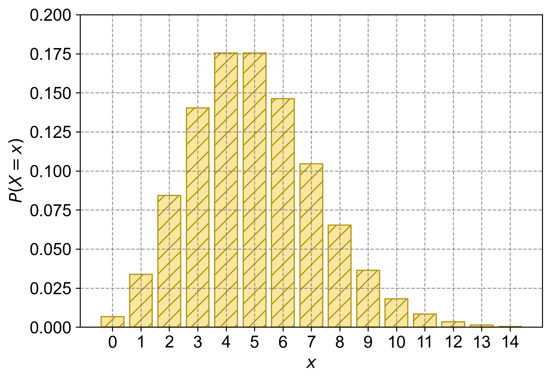
The low probability of finding no wildflowers (0.67%) aligns with the relatively high average rate (\(\lambda = 5\)).
The high probability of finding at least one wildflower (99.33%) suggests that these flowers are common in this meadow.
The relatively low probability (12.47%) for at most two flowers indicates that it’s more likely to find more than two flowers per square meter.

Fig. 4.22 The probability mass function (PMF) for a Poisson distribution with \(\lambda = 5\). Each bar represents the probability of observing exactly \(x\) flowers per square meter.#
Example 4.28
In a small town, historical data shows that the average number of power outages per year is 2. Using this information:
a. Calculate the probability of experiencing no power outages in a given year.
b. Determine the probability of experiencing at least one power outage in a year.
c. Compute the probability of experiencing more than three power outages in a year.
d. What is the most likely number of power outages to occur in a year?
Solution: Let X represent the number of power outages in a year. We can model this situation using a Poisson distribution because:
Power outages are relatively rare events occurring over a fixed time period (one year).
Each outage occurs independently of others.
We know the average rate of occurrence (\(\lambda = 2\) outages per year).
The Poisson probability mass function is:
where \(\lambda\) is the average rate (2 outages per year) and k is the number of outages we’re interested in.
a. To find the probability of no power outages in a year:
We use k = 0 in the Poisson probability mass function:
This means there’s about a 13.53% chance of experiencing no power outages in a given year.
b. For the probability of experiencing at least one power outage:
We use the complement rule:
This indicates a high probability (about 86.47%) of experiencing at least one power outage in a year.
c. To compute the probability of experiencing more than three power outages:
We’ll use the complement rule again, calculating the probability of 3 or fewer outages and subtracting from 1:
This shows there’s about a 14.29% chance of experiencing more than three power outages in a year.
d. To find the most likely number of power outages:
In a Poisson distribution, the expected value (mean) is equal to the parameter \(\lambda\). In this case, \(\lambda = 2\), so the expected number of power outages in a year is 2.
We can explore this concept further:
Expected Value: \(E(X) = \lambda = 2\). This means that, on average, we expect 2 power outages per year.
Variance: \(Var(X) = \lambda = 2\). The variance being equal to the mean is a unique property of the Poisson distribution.
Standard Deviation: \(SD(X) = \sqrt{\lambda} \approx 1.414\). This tells us about the typical deviation from the mean.
We can calculate probabilities around this expected value:
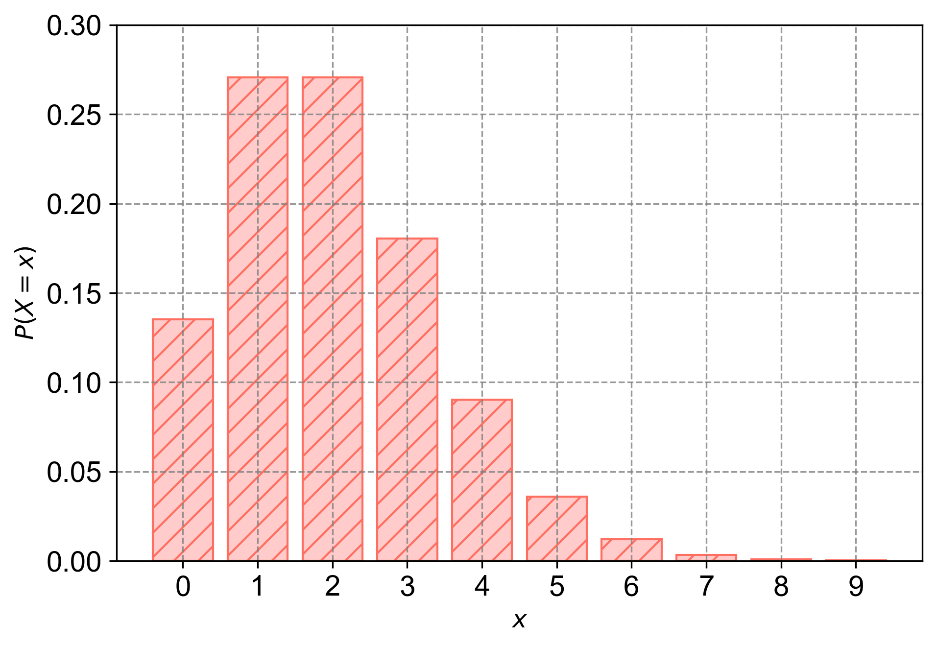
We see that \(P(X = 1)\) and \(P(X = 2)\) are equal and higher than \(P(X = 3)\), which aligns with our expected value of 2.
Interpretation of results:
The expected number of power outages per year is 2, which gives us a central point for planning and analysis.
There’s a relatively low chance (13.53%) of having a year without any power outages, which is less than the expected value.
It’s highly likely (86.47%) that the town will experience at least one power outage in a year, which is consistent with the positive expected value.
The probability of having more than three outages (14.29%) is lower than having two or fewer, which aligns with the expected value of 2.
The standard deviation of about 1.414 suggests that it’s not uncommon for the actual number of outages to deviate from the expected value by 1 or 2.

Fig. 4.23 The probability mass function (PMF) for a Poisson distribution with \(\lambda = 2\). Each bar represents the probability of observing exactly \(x\) power outages per year.#
Example 4.29
A customer service department receives an average of 20 emails per hour. Assuming that the Poisson distribution is appropriate for modeling the number of emails received:
a. Calculate the probability of receiving exactly 15 emails in a randomly selected hour.
b. Determine the probability of receiving exactly 25 emails in an hour.
c. What is the probability of receiving 20 or fewer emails in an hour?
d. Calculate the expected number of emails in a 4-hour period.
Solution: Let \(X\) represent the number of emails received in an hour. We model this using a Poisson distribution with parameter \(\lambda = 20\) (the average number of emails per hour).
The Poisson probability mass function is:
where \(\lambda\) is the average rate (20 emails per hour) and \(k\) is the number of emails we’re interested in.
a. For exactly 15 emails in an hour:
This means there’s about a 5.16% chance of receiving exactly 15 emails in a randomly selected hour.
b. For exactly 25 emails in an hour:
This indicates approximately a 4.46% chance of receiving exactly 25 emails in an hour.
c. To find the probability of receiving 20 or fewer emails in an hour:
We need to sum the probabilities for \(X = 0\) to \(X = 20\):
This shows there’s about a 55.91% chance of receiving 20 or fewer emails in an hour.
d. For the expected number of emails in a 4-hour period:
The Poisson distribution has the property that the expected value \(E(X) = \lambda\). For a 4-hour period, we multiply the hourly rate by 4:
Interpretation:
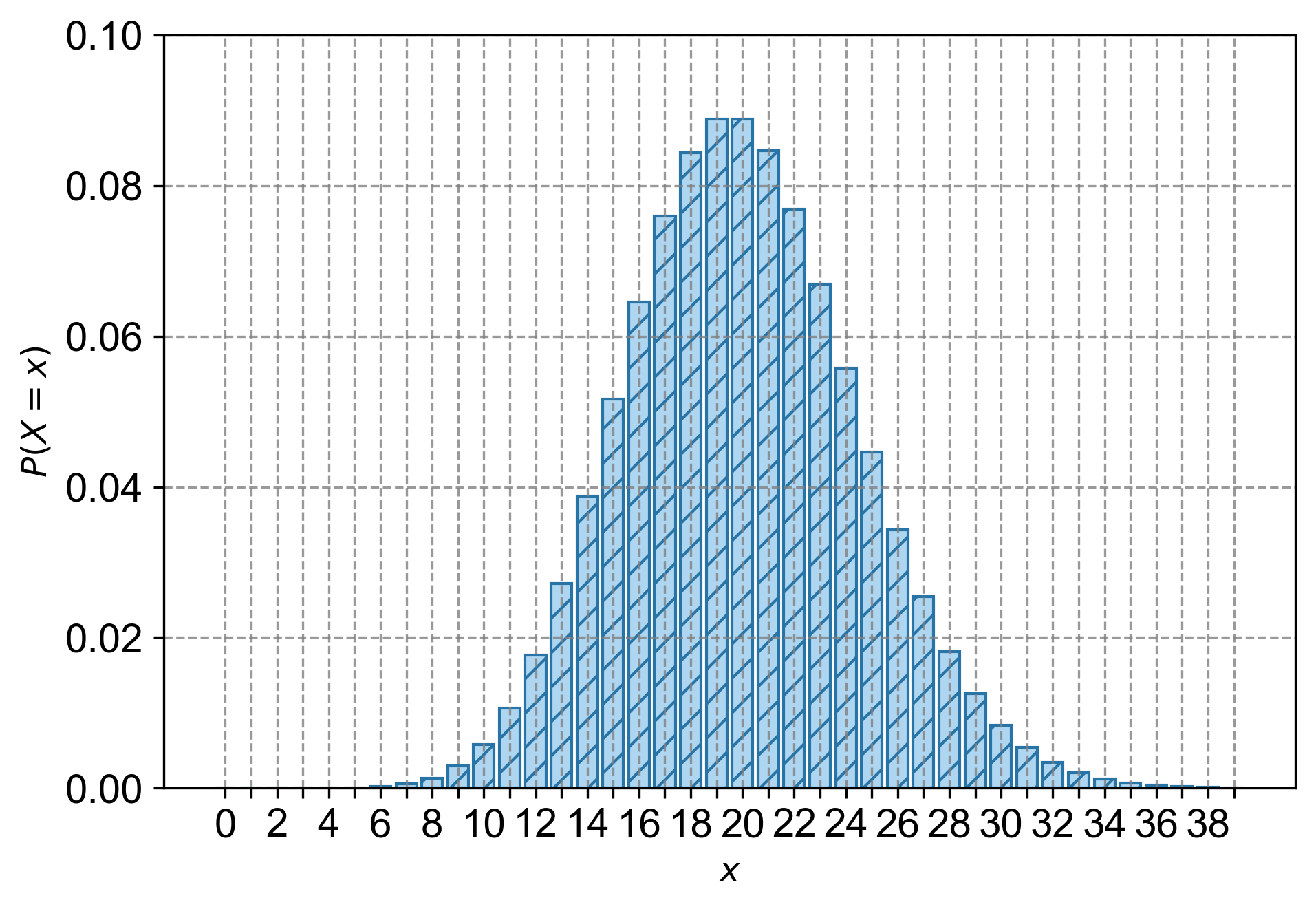
The probability of receiving exactly 15 emails (5.16%) is slightly higher than receiving exactly 25 emails (4.46%), reflecting that 15 is closer to the mean (\(\mu=20\)).
There’s about a 55.91% chance of receiving 20 or fewer emails, meaning there’s about a 44.09% chance of receiving more than 20.
The expected number of emails over a 4-hour period is 80, which can help plan staffing levels for longer shifts.

Fig. 4.24 The probability mass function (PMF) for a Poisson distribution with \(\lambda = 20\). Each bar represents the probability of observing exactly \(x\) emails per hour, where \(x\) ranges from \(0\) to \(30\).#
4.4.1. Poisson Distribution as an Approximation to the Binomial Distribution#
The Poisson distribution can serve as an approximation for the binomial distribution under certain conditions, typically when the number of trials \(n\) is large, and the probability of success \(p\) in each trial is small. This approximation is particularly useful because it simplifies calculations when dealing with large \(n\).
Criteria for Using the Poisson Approximation
The Poisson approximation to the binomial distribution is most appropriate when the following two criteria are met:
The number of trials \(n\) is large (\(n \geq 100\)).
The product of the number of trials and the probability of success (\(np\)) is small (\(np \leq 10\)).
Mean of the Poisson Approximation
When using the Poisson distribution to approximate a binomial distribution, the mean \(\mu\) of the Poisson distribution is set to be equal to the product of the number of trials and the probability of success:
This mean \(\mu\) is then used as the parameter \(\lambda\) for the Poisson distribution.
Example 4.30
In a large office, the rate of employees catching a common cold during the winter season is \(3\%\). If \(150\) employees are randomly selected, calculate the probability of at least one employee catching a common cold.
Solution: This problem involves a binomial scenario (each employee either catches a cold or doesn’t), but we can approximate it using a Poisson distribution due to the large number of employees and the low probability of catching a cold.
First, let’s check if we can use the Poisson approximation:
Number of trials: \(n = 150\) (employees)
Probability of success: \(p = 0.03\) (\(3\%\) chance of catching a cold)
We need: \(n \geq 100\) and \(np \leq 10\)
We have: \(150 \geq 100\) and \(150 \cdot 0.03 = 4.5 \leq 10\) So, we can use the Poisson approximation.
Calculate \(\lambda\) for the Poisson distribution:
\[\begin{equation*} \lambda = np = 150 \cdot 0.03 = 4.5 \end{equation*}\]In a Poisson distribution, \(\lambda\) represents the average number of occurrences. Here, it means we expect an average of \(4.5\) employees to catch a cold.
To find the probability of at least one employee catching a cold, we can use the complement rule:
\[\begin{equation*}P(\text{at least one}) = 1 - P(\text{none})\end{equation*}\]Calculate \(P(X = 0)\) using the Poisson probability mass function:
\[\begin{equation*}P(X = k) = \dfrac{e^{-\lambda} \lambda^k}{k!}\end{equation*}\]\[\begin{equation*}P(X = 0) = \dfrac{e^{-4.5} 4.5^0}{0!} = \dfrac{e^{-4.5} \cdot 1}{1} = e^{-4.5} \approx 0.0111\end{equation*}\]Therefore, the probability of at least one employee catching a cold is:
\[\begin{equation*}P(\text{at least one}) = 1 - P(\text{none}) = 1 - 0.0111 \approx 0.9889\end{equation*}\]
Interpretation: There is approximately a \(98.89\%\) chance that at least one employee out of \(150\) will catch a common cold during the winter season. This high probability is not surprising given that we expect an average of \(4.5\) employees to catch a cold.
Note
The Poisson approximation is particularly useful here because it simplifies the calculation. If we were to use the exact binomial probability, we would need to calculate:
This calculation represents the probability of at least one success in 150 trials, where each trial has a 97% chance of failure (3% chance of success). Here’s why:
\((0.97)^{150}\) is the probability of all 150 employees not catching a cold.
\(1 - (0.97)^{150}\) is therefore the probability of at least one employee catching a cold.
This binomial calculation is more computationally intensive, especially without a calculator. The Poisson approximation gives us a very close result with simpler calculations.
Example 4.31
In a certain city, the rate of a specific traffic incident is 2%. If 200 cars are randomly selected, find the probability of at least one car being involved in the incident.
Solution: Let’s approach this step-by-step:
Given information:
Number of trials (cars): \(n = 200\)
Probability of the incident for each car: \(p = 0.02\) (2%)
Check if we can use the Poisson approximation:
We need: \(n \geq 100\) and \(np \leq 10\)
We have: \(200 \geq 100\) and \(200 \cdot 0.02 = 4 \leq 10\) Both conditions are satisfied, so we can use the Poisson approximation.
Calculate \(\lambda\) for the Poisson distribution:
\[\begin{equation*}\lambda = np = 200 \cdot 0.02 = 4\end{equation*}\]This \(\lambda\) represents the average number of cars expected to be involved in the incident.
In a Poisson distribution, the probability of exactly \(k\) occurrences is given by:
\[\begin{equation*}P(X = k) = \dfrac{e^{-\lambda} \lambda^k}{k!}\end{equation*}\]We want the probability of at least one car being involved. We can calculate this as:
\[\begin{equation*}P(\text{at least one}) = 1 - P(\text{none})\end{equation*}\]Calculate \(P(X = 0)\) using the Poisson probability mass function:
\[\begin{equation*}P(X = 0) = \dfrac{e^{-4} 4^0}{0!} = e^{-4} \approx 0.0183\end{equation*}\]Therefore, the probability of at least one car being involved is:
\[\begin{equation*}P(\text{at least one}) = 1 - P(\text{none}) = 1 - 0.0183 \approx 0.9817\end{equation*}\]
Interpretation: There is approximately a 98.17% chance that at least one car out of 200 will be involved in the specific traffic incident. This high probability is consistent with the expected average of 4 cars being involved.
Example 4.32
In a local community, the rate of rare plant species being found is 1%. If 300 plants are randomly surveyed, find the probability of discovering at least one of these rare species.
Solution:
Let’s approach this problem step-by-step:
Given information:
Number of plants surveyed: \(n = 300\)
Probability of a plant being a rare species: \(p = 0.01\) (1%)
Check if we can use the Poisson approximation:
We need: \(n \geq 100\) and \(np \leq 10\)
We have: \(300 \geq 100\) and \(300 \cdot 0.01 = 3 \leq 10\) Both conditions are satisfied, so we can use the Poisson approximation.
Calculate \(\lambda\) for the Poisson distribution:
\[\begin{equation*}\lambda = np = 300 \cdot 0.01 = 3\end{equation*}\]This \(\lambda\) represents the average number of rare plant species expected to be found in the survey.
In a Poisson distribution, the probability of exactly \(k\) occurrences is given by:
\[\begin{equation*}P(X = k) = \dfrac{e^{-\lambda} \lambda^k}{k!}\end{equation*}\]We want the probability of discovering at least one rare species. We can calculate this as:
\[\begin{equation*}P(\text{at least one}) = 1 - P(\text{none})\end{equation*}\]Calculate \(P(X = 0)\) using the Poisson probability mass function:
\[\begin{equation*}P(X = 0) = \dfrac{e^{-3} 3^0}{0!} = e^{-3} \approx 0.0498\end{equation*}\]Therefore, the probability of discovering at least one rare species is:
\[\begin{equation*}P(\text{at least one}) = 1 - P(\text{none}) = 1 - 0.0498 \approx 0.9502\end{equation*}\]
Interpretation: There is approximately a 95.02% chance of discovering at least one rare plant species in a survey of 300 plants. This high probability is consistent with the expected average of 3 rare species being found in the survey.
Example 4.33
A large online retailer receives an average of 8 customer service inquiries per hour. Assume the number of inquiries follows a Poisson distribution.
a) What is the probability of receiving exactly 5 inquiries in a given hour?
b) What is the probability of receiving 10 or more inquiries in a given hour?
c) What is the probability of receiving fewer than 3 inquiries in a given hour?
d) If the customer service team can handle up to 12 inquiries per hour without delays, what is the probability that they will experience delays in a given hour?
e) What is the expected number of inquiries in a 30-minute period?
Solution: Let \(X\) be the number of customer service inquiries per hour. Then X ~ Poisson(\(\lambda\) = 8).
a) The probability of receiving exactly 5 inquiries in a given hour:
b) The probability of receiving 10 or more inquiries in a given hour:
c) The probability of receiving fewer than 3 inquiries in a given hour:
d) The probability that the customer service team will experience delays in a given hour:
e) For a Poisson distribution, we know that \(\mu = \lambda = np\), where \(n\) is the number of trials and \(p\) is the probability of success for each trial. In this case, \(\lambda = 8\) inquiries per hour.
For a 30-minute period, we need to adjust \(\lambda\) because we’re dealing with half an hour instead of a full hour:
The expected number of inquiries in a 30-minute period is equal to \(\lambda_{30\text{ min}}\):
This means that, on average, we expect 4 customer service inquiries in a 30-minute period.
Example 4.34
A call center receives an average of 12 customer service calls per hour. Assume the number of calls follows a Poisson distribution.
a) What is the probability of receiving exactly 15 calls in a given hour?
b) What is the probability of receiving 10 or fewer calls in a given hour?
c) What is the probability of receiving more than 20 calls in a given hour?
d) What is the expected number of calls in a 30-minute period?
e) If the call center has 3 operators, each able to handle up to 5 calls per hour, what is the probability that they will be overwhelmed (i.e., receive more than 15 calls) in a given hour?
Solution: Let X be the number of customer service calls per hour. Then X ~ Poisson(λ = 12).
a) The probability of receiving exactly 15 calls in a given hour:
b) The probability of receiving 10 or fewer calls in a given hour:
c) The probability of receiving more than 20 calls in a given hour:
d) For a 30-minute period, we need to adjust λ:
The expected number of calls in 30 minutes is:
e) The probability of receiving more than 15 calls in a given hour:
This means there’s approximately a 15.56% chance that the call center will be overwhelmed in a given hour.
Note that the individual probabilities for X ≤ 10 provide insight into the distribution of calls:
These probabilities show that it’s most likely to receive around 10-14 calls per hour, which aligns with the average of 12 calls per hour.
