7.8. Hypothesis Tests for One Population Mean When \(\sigma\) Is Unknown#
When conducting hypothesis tests involving a single population mean, the procedure varies based on whether the population standard deviation (\(\sigma\)) is known. This section outlines the procedure for cases where \(\sigma\) is unknown, utilizing the t-test to evaluate hypotheses about the population mean.
Algorithm 7.2 (Hypothesis Tests for One Population Mean with Unknown Standard Deviation)
Objective: To conduct a hypothesis test for the population mean (\(\mu\)) when the population standard deviation (\(\sigma\)) is unknown.
Prerequisites:
A simple random sample is obtained.
The population is normally distributed or the sample size is sufficiently large.
The population standard deviation (\(\sigma\)) is unknown.
Method:
Define the Significance Level: Choose the significance level (\(\alpha\)).
State the Hypotheses:
Two-Tailed Test:
Null Hypothesis: \(H_0: \mu = \mu_{0}\)
Alternative Hypothesis: \(H_a: \mu \neq \mu_{0}\)
Left-Tailed Test:
Null Hypothesis: \(H_0: \mu \geq \mu_{0}\)
Alternative Hypothesis: \(H_a: \mu < \mu_{0}\)
Right-Tailed Test:
Null Hypothesis: \(H_0: \mu \leq \mu_{0}\)
Alternative Hypothesis: \(H_a: \mu > \mu_{0}\)
Calculate the Test Statistic: Use the formula:
(7.15)#\[\begin{equation} t = \dfrac{\overline{x} - \mu_{0}}{\dfrac{s}{\sqrt{n}}} \end{equation}\]where \(\overline{x}\) is the sample mean, \(s\) is the sample standard deviation, and \(n\) is the sample size.
Determine Critical Value(s):
For two-tailed tests: \(\pm t_{\alpha/2, \, df}\)
For left-tailed tests: \(-t_{\alpha, \, df}\)
For right-tailed tests: \(t_{\alpha, \, df}\)
where \(df\) (degrees of freedom) = \(n - 1\).
Decision Rule:
Critical-Value Approach:
If the test statistic falls within the rejection region, reject \(H_0\); otherwise, do not reject \(H_0\).
P-value Approach:
Calculate the p-value using the test statistic.
Reject \(H_0\) if \(p \leq \alpha\); otherwise, do not reject \(H_0\).
This algorithm outlines the steps to perform a hypothesis test for a population mean when the population standard deviation is unknown. Using the t-distribution ensures appropriate handling of the additional uncertainty due to estimating the population standard deviation, leading to valid conclusions about the population mean.
Example 7.33
A nutritionist claims that a new diet program can reduce the average cholesterol level in adults to below 200 mg/dL. To test this claim, a random sample of 12 adults following the diet was tested, and the following cholesterol levels (in mg/dL) were recorded:
At the 5% significance level, do the data provide sufficient evidence to conclude that the mean cholesterol level for adults on this diet is less than 200 mg/dL? Assume that the population standard deviation of cholesterol levels is unknown.
Solution:
Hypothesis Test:
Null Hypothesis (\(H_0\)): \(\mu \geq 200\) mg/dL
Alternative Hypothesis (\(H_a\)): \(\mu < 200\) mg/dL
Sample Statistics:
\(n = 12\)
\(\overline{x} = 197.42\) mg/dL (calculated as the mean of the sample data)
\(s = 7.07\) mg/dL (sample standard deviation)
Significance Level: \(\alpha = 0.05\)
Test Statistic:
Degrees of Freedom: \(df = n - 1 = 11\)
Critical-Value Approach:
Critical value: \(t_{\alpha, df} = t_{0.05, 11} \approx -1.796\)
Since \(\text{Test Statistic} = -1.00 > t_{0.05, 11} = -1.796\), do not reject \(H_0\).
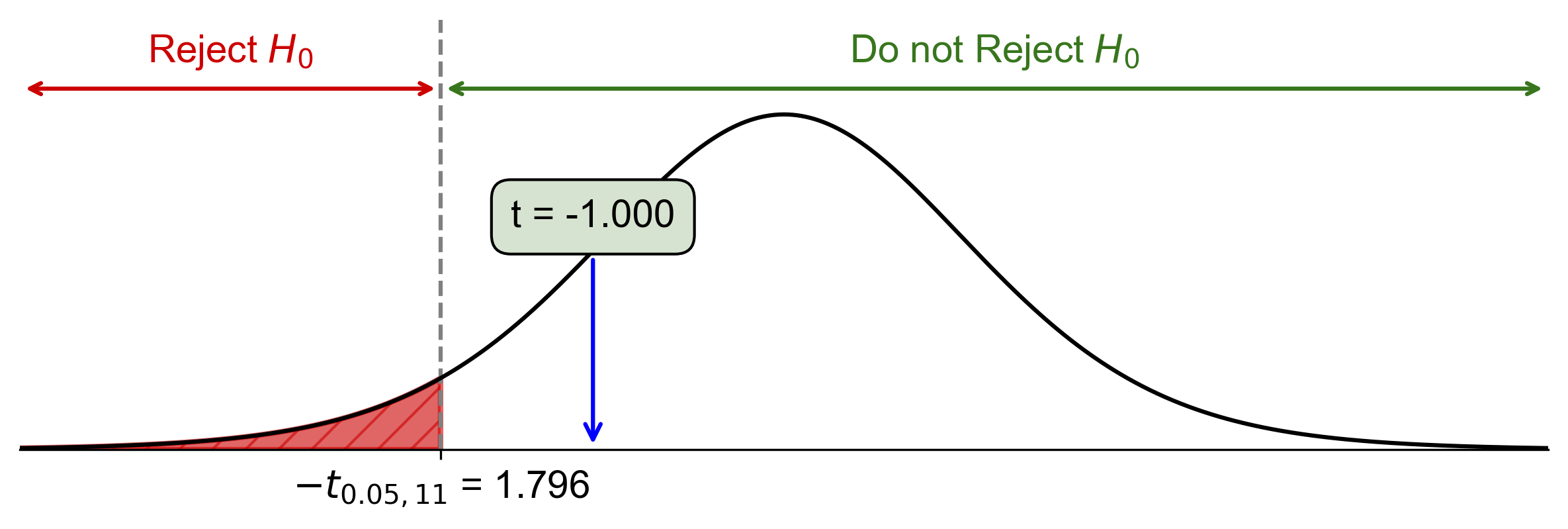
Fig. 7.36 Critical-value approach illustrating the rejection region and test statistic for Example 7.33.#
P-Value Approach:
Calculated P-Value: \(P(T < -1.00) \approx 0.1694\)
Since \(\text{P-value} = 0.1694 > \alpha = 0.05\), do not reject \(H_0\).
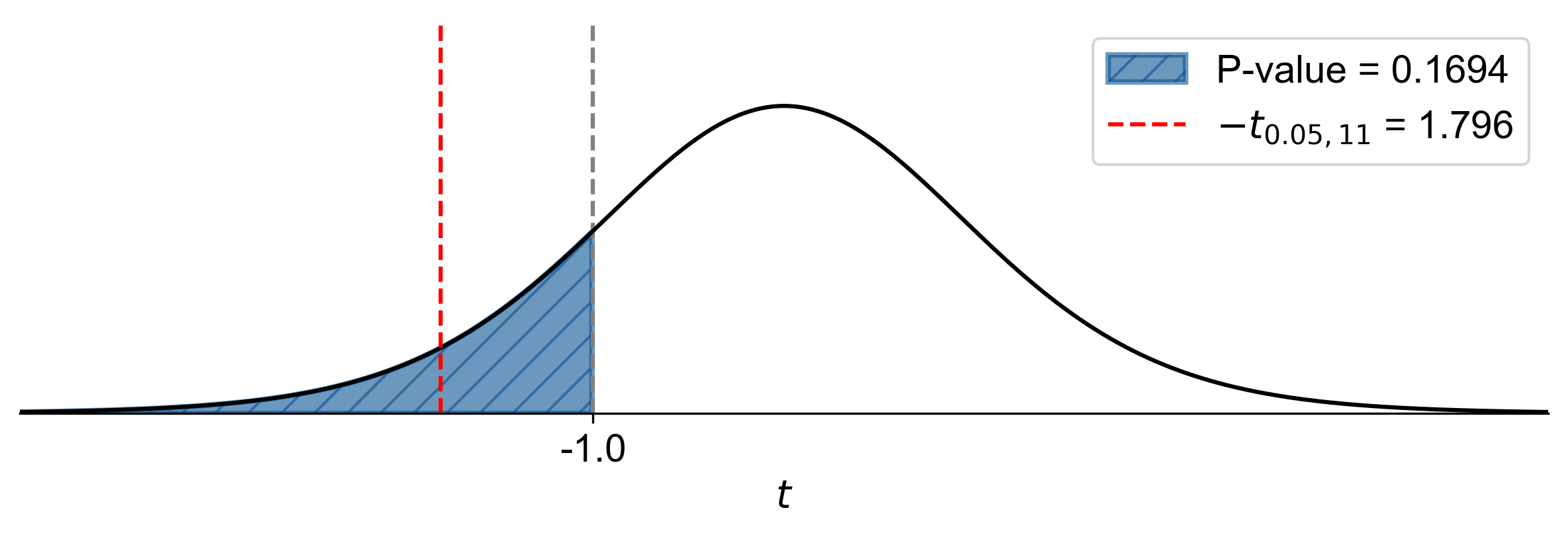
Fig. 7.37 P-value approach demonstrating the significance of the test statistic in relation to the null hypothesis for Example 7.33.#
Approximating P-Value Using the T-Distribution Table: We can also approximate the p-value using the t-distribution table for degrees of freedom (df = 11):
Area in One Tail
Critical t-Value (df = 11)
0.1
1.363
0.05
1.796
0.025
2.201
0.01
2.718
0.005
3.106
0.001
4.025
Given that our test statistic of approximately \(|-1|=1\) is less than 1.363, we can infer that: The p-value is greater than 0.1.
Since \(\text{P-value} > 0.1 > \alpha = 0.05\), do not reject \(H_0\).
Conclusion: At the 5% significance level, the data do not provide sufficient evidence to conclude that the mean cholesterol level for adults on this diet is less than 200 mg/dL.
The figures illustrate both the critical-value and p-value approaches, providing a visual representation of the hypothesis test results.
Example 7.34
A dietitian claims that a new supplement can increase the average daily protein intake of individuals to above 70 grams. To test this claim, a random sample of 10 individuals who took the supplement was tested, and the following protein intakes (in grams) were recorded:
At the 5% significance level, do the data provide sufficient evidence to conclude that the mean daily protein intake for individuals taking this supplement is greater than 70 grams? Assume that the population standard deviation of protein intakes is unknown.
Solution:
Hypothesis Test:
Null Hypothesis (\(H_0\)): \(\mu \leq 70\) grams
Alternative Hypothesis (\(H_a\)): \(\mu > 70\) grams
Sample Statistics:
\(n = 10\)
\(\overline{x} = 72.3\) grams (calculated as the mean of the sample data)
\(s = 3.82\) grams (sample standard deviation)
Significance Level: \(\alpha = 0.05\)
Test Statistic:
Degrees of Freedom: \(df = n - 1 = 9\)
Critical-Value Approach:
Critical value: \(t_{\alpha, df} = t_{0.05, 9} \approx 1.833\)
Since \(\text{Test Statistic} = 1.975 > t_{0.05, 9} = 1.833\), reject \(H_0\).
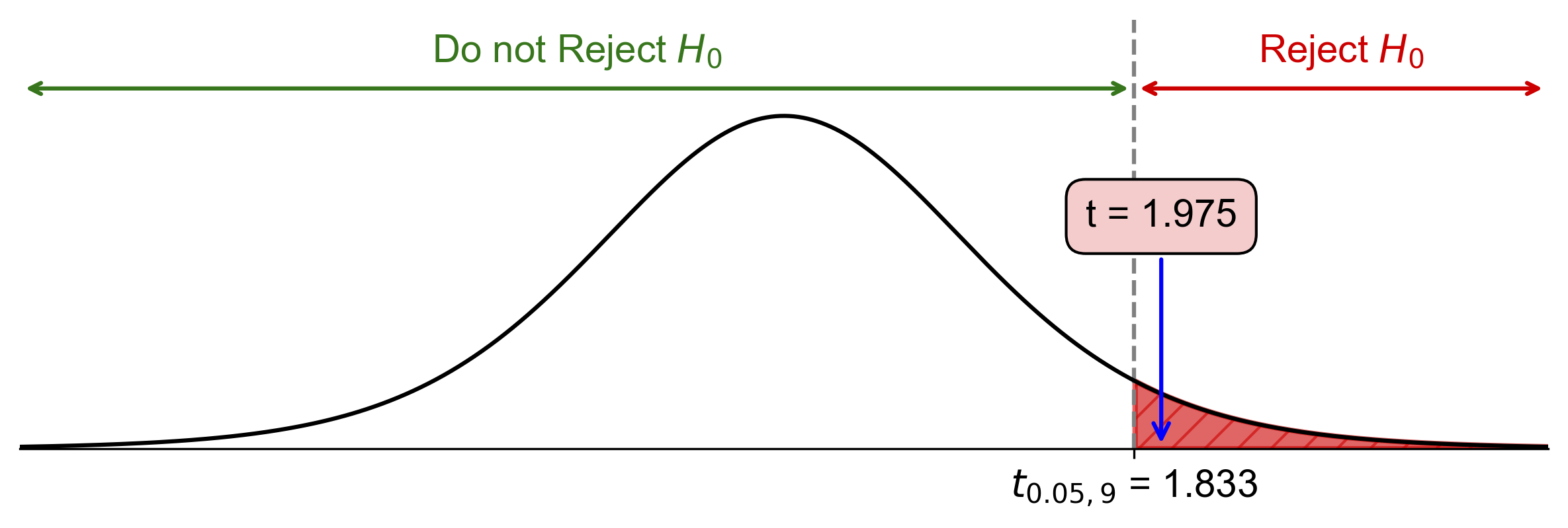
Fig. 7.38 Critical-value approach illustrating the rejection region and test statistic for Example 7.34.#
P-Value Approach:
Calculated P-Value: Using statistical software, we find: \( P(T > 1.975) \approx 0.0399 \)
Since \(\text{P-value} = 0.0399 < \alpha = 0.05 \), reject \(H_0 \).
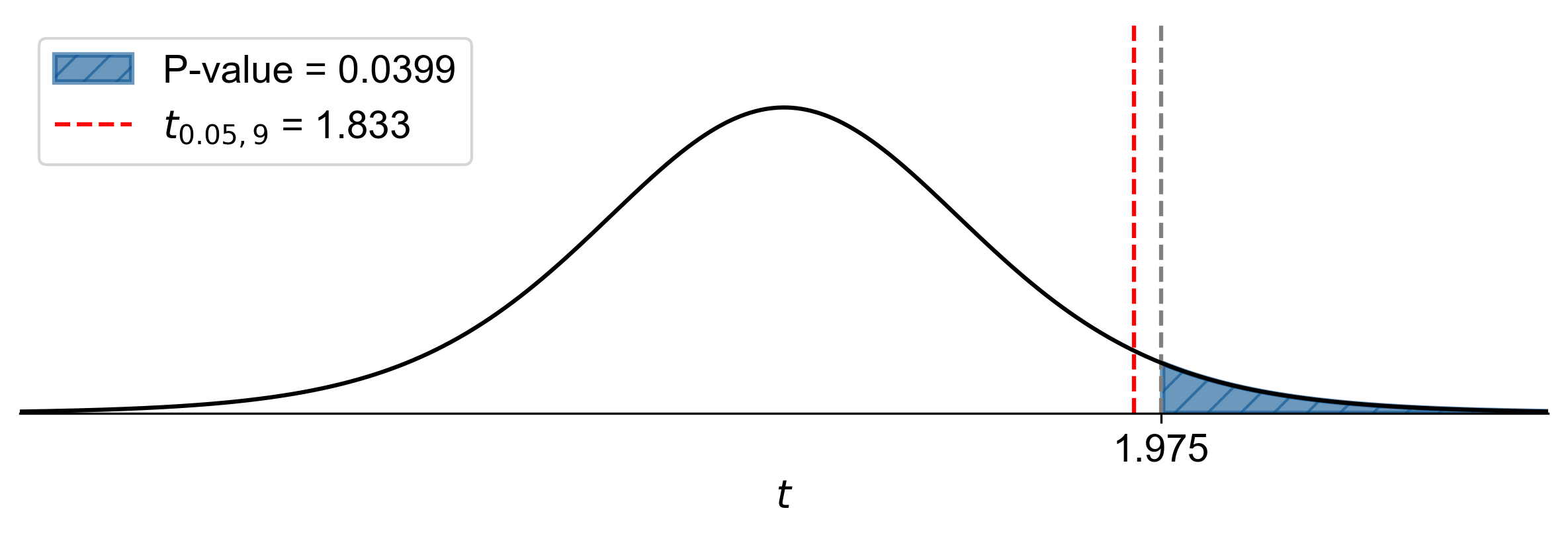
Fig. 7.39 P-value approach demonstrating the significance of the test statistic in relation to the null hypothesis for Example 7.33.#
Approximating P-Value Using the T-Distribution Table: We can also approximate the p-value using the t-distribution table for degrees of freedom (df = 9):
Area in One Tail
Critical t-Value (df = 9)
0.10
1.383
0.05
1.833
0.025
2.262
0.01
2.821
0.005
3.250
0.001
4.297
Given that our test statistic of approximately 1.975 is between 1.833 and 2.262, we can infer that: The p-value is between 0.05 and 0.025, which supports our earlier calculation.
Conclusion: At the 5% significance level, the data provide sufficient evidence to conclude that the mean daily protein intake for individuals taking this supplement is greater than 70 grams.
Example 7.35
A fitness coach claims that a new training program can reduce the average heart rate of participants to below 200 beats per minute (bpm) after a workout session. To test this claim, a random sample of 13 individuals who completed the training program was monitored, and the following heart rates (in bpm) were recorded:
At the 5% significance level, do the data provide sufficient evidence to conclude that the mean heart rate for individuals following this training program is less than 200 bpm? Assume that the population standard deviation of heart rates is unknown.
Solution:
Hypothesis Test:
Null Hypothesis (\(H_0\)): \(\mu \geq 200\) bpm
Alternative Hypothesis (\(H_a\)): \(\mu < 200\) bpm
Sample Statistics:
\(n = 13\)
\(\overline{x} = 197.538\) bpm (calculated as the mean of the sample data)
\(s = 7.501\) bpm (sample standard deviation)
Significance Level: \(\alpha = 0.05\)
Test Statistic:
Degrees of Freedom: \(df = n - 1 = 12\)
Critical-Value Approach:
Critical value: \(t_{\alpha, df} = t_{0.05, 12} \approx -1.782\)
Since \(\text{Test Statistic} = -1.183 > t_{0.05, 12} = -1.782\), do not reject \(H_0\).
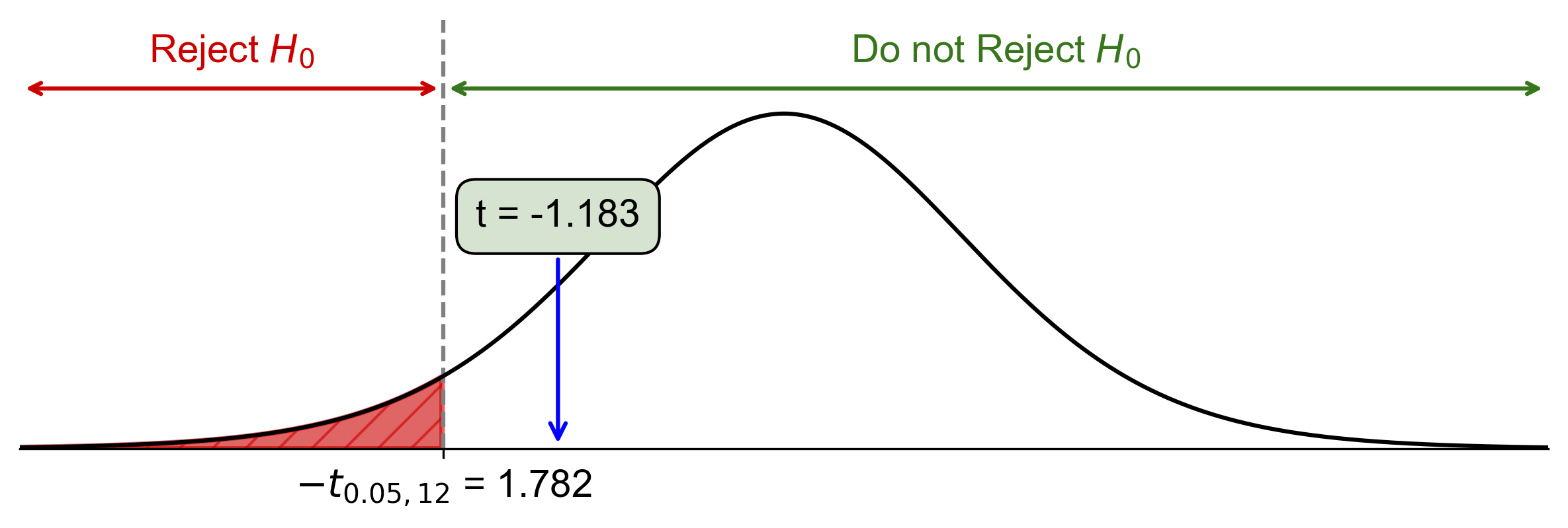
Fig. 7.40 Critical-value approach illustrating the rejection region and test statistic for Example 7.35.#
P-Value Approach:
Calculated P-Value: \(P(T < -1.183) \approx 0.1298\)
Since \(\text{P-value} = 0.1298 > \alpha = 0.05\), do not reject \(H_0\).
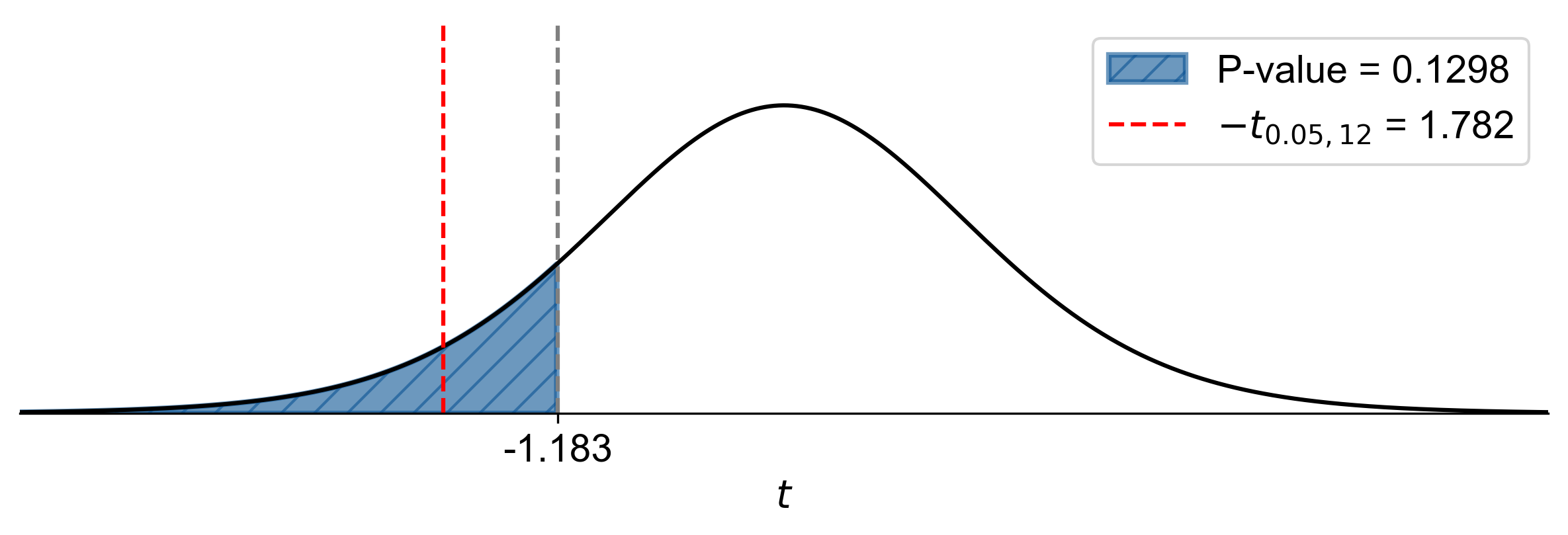
Fig. 7.41 P-value approach demonstrating the significance of the test statistic in relation to the null hypothesis for Example 7.35.#
Approximating P-Value Using the T-Distribution Table: We can also approximate the p-value using the t-distribution table for degrees of freedom (df = 12):
Area in One Tail
Critical t-Value (df = 12)
0.1
1.356
0.05
1.782
0.025
2.179
0.01
2.681
0.005
3.055
0.001
3.930
Given that our test statistic of approximately \(|-1.183|=1.183\) is less than 1.356, we can infer that: The p-value is greater than 0.1.
Since \(\text{P-value} > 0.1 > \alpha = 0.05\), do not reject \(H_0\).
Conclusion: At the 5% significance level, the data do not provide sufficient evidence to conclude that the mean heart rate for individuals following this training program is less than 200 bpm.
Example 7.36
A biologist claims that the mean weight of a certain species of fish in a lake is 5 kg. To test this claim, a random sample of 15 fish was caught, and their weights (in kg) were recorded as follows:
At the 5% significance level, do the data provide sufficient evidence to conclude that the mean weight of this species of fish in the lake is different from 5 kg? Assume that the population standard deviation of fish weights is unknown.
Solution:
Hypothesis Test:
Null Hypothesis (\(H_0\)): \(\mu = 5\) kg
Alternative Hypothesis (\(H_a\)): \(\mu \neq 5\) kg
Sample Statistics:
\(n = 15\)
\(\overline{x} = 5.03\) kg (calculated as the mean of the sample data)
\(s = 0.198\) kg (sample standard deviation)
Significance Level: \(\alpha = 0.05\)
Test Statistic:
Degrees of Freedom: \(df = n - 1 = 14\)
Critical-Value Approach:
Critical value: \(t_{\alpha/2, df} = t_{0.025, 14} \approx \pm 2.145\)
Since \(\text{Test Statistic} = 0.521\) is within the range \(-2.145 < t < 2.145\), fail to reject \(H_0\).
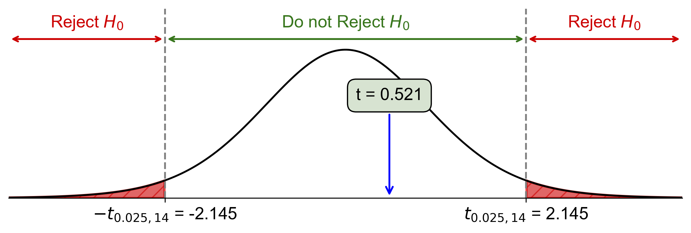
Fig. 7.42 Critical-value approach illustrating the rejection region and test statistic for Example 7.36.#
P-Value Approach:
Calculated P-Value: \(2 \times P(T > 0.521) \approx 0.6102\)
Since \(\text{P-value} = 0.6102 > \alpha = 0.05\), fail to reject \(H_0\).
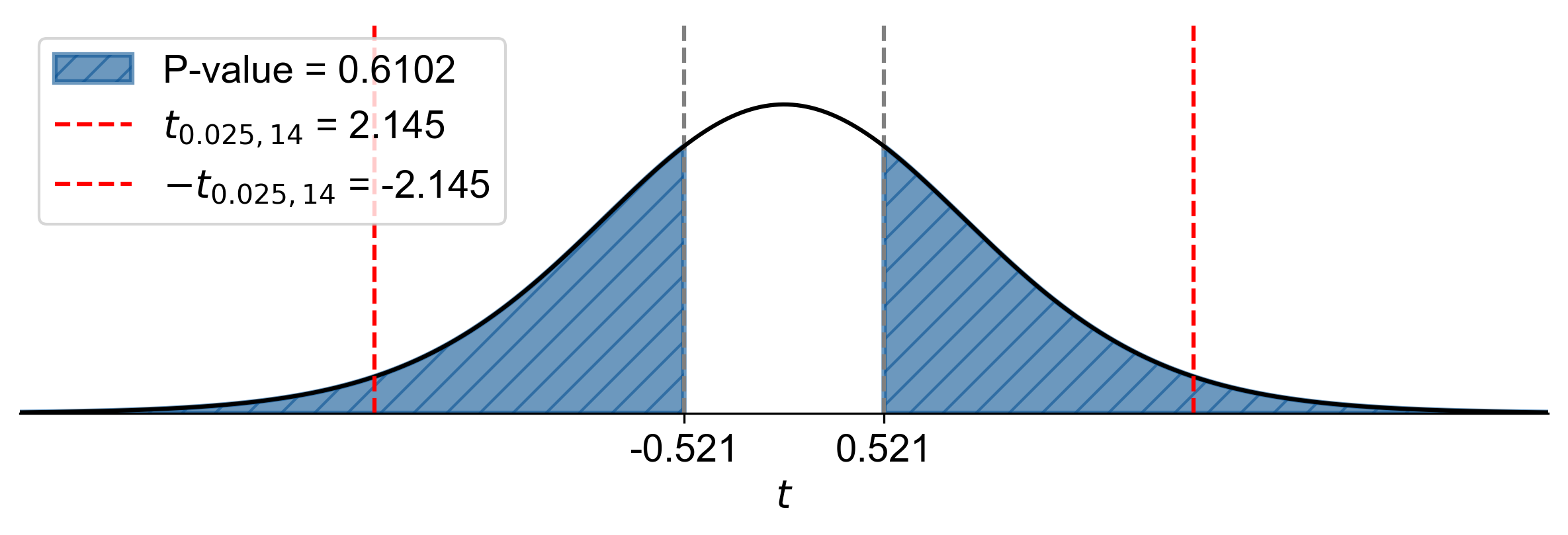
Fig. 7.43 P-value approach demonstrating the significance of the test statistic in relation to the null hypothesis for Example 7.36.#
Approximating P-Value Using the T-Distribution Table: We can also approximate the p-value using the t-distribution table for degrees of freedom (df = 14):
Area in One Tail
Critical t-Value (df = 14)
0.1
1.345
0.05
1.761
0.025
2.145
0.01
2.624
0.005
2.977
0.001
3.787
Given that our test statistic of 0.521 is less than 1.345, we can infer that: The p-value is greater than 0.2 (for a two-tailed test).
Since \(\text{P-value} > 0.2 > \alpha = 0.05\), fail to reject \(H_0\).
Conclusion: At the 5% significance level, the data do not provide sufficient evidence to conclude that the mean weight of this species of fish in the lake is different from 5 kg.
Example 7.37
A researcher claims that a new drug can lower the average systolic blood pressure in patients with hypertension to below 140 mmHg. To test this claim, a random sample of 15 patients using the drug was tested, and the following systolic blood pressure readings (in mmHg) were recorded:
At the 5% significance level, do the data provide sufficient evidence to conclude that the mean systolic blood pressure for patients using this drug is less than 140 mmHg? Assume that the population standard deviation of systolic blood pressure is unknown.
Solution:
Hypothesis Test:
Null Hypothesis (\(H_0\)): \(\mu \geq 140\) mmHg
Alternative Hypothesis (\(H_a\)): \(\mu < 140\) mmHg
Sample Statistics:
\(n = 15\)
\(\overline{x} = 139.53\) mmHg (calculated as the mean of the sample data)
\(s = 3.02\) mmHg (sample standard deviation)
Significance Level: \(\alpha = 0.05\)
Test Statistic:
Degrees of Freedom: \(df = n - 1 = 14\)
Critical-Value Approach:
Critical value: \(t_{\alpha, df} = t_{0.05, 14} \approx -1.761\)
Since \(\text{Test Statistic} = -0.598 > t_{0.05, 14} = -1.761\), do not reject \(H_0\).
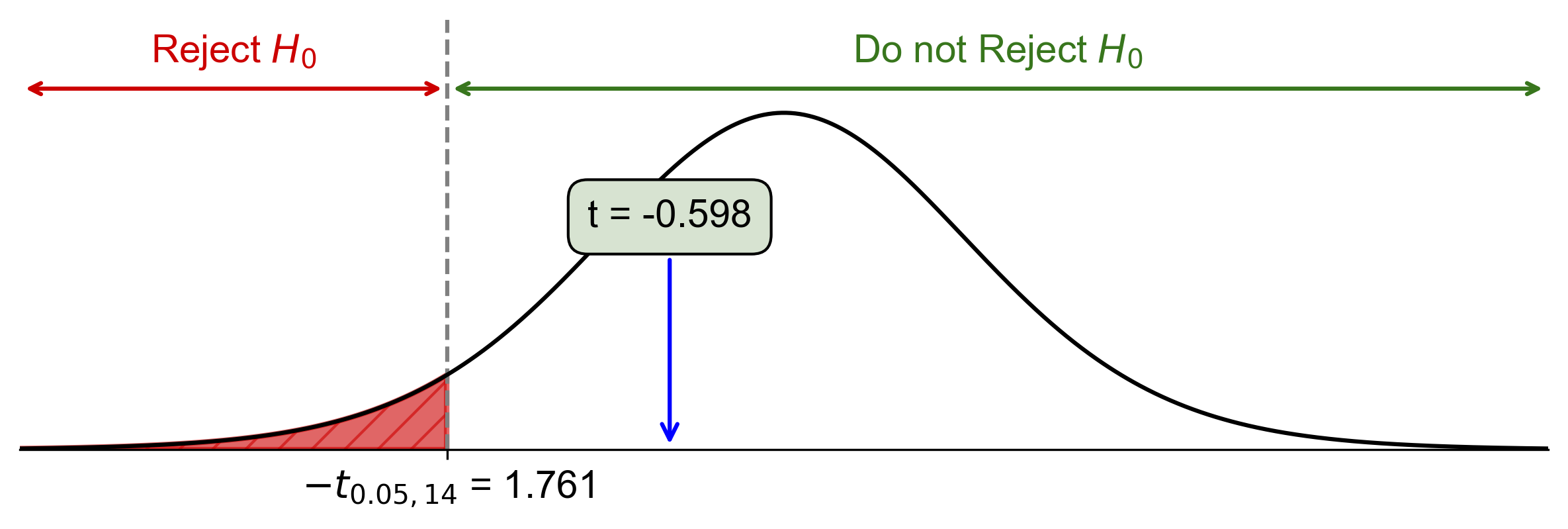
Fig. 7.44 Critical-value approach illustrating the rejection region and test statistic for Example 7.37.#
P-Value Approach:
Calculated P-Value: \(P(T < -0.598) \approx 0.2796\)
Since \(\text{P-value} = 0.2796 > \alpha = 0.05\), do not reject \(H_0\).
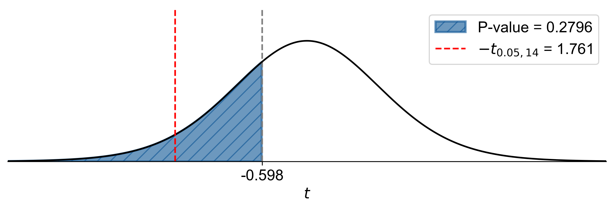
Fig. 7.45 P-value approach demonstrating the significance of the test statistic in relation to the null hypothesis for Example 7.37.#
Approximating P-Value Using the T-Distribution Table: We can also approximate the p-value using the t-distribution table for degrees of freedom (df = 14):
Area in One Tail
Critical t-Value (df = 14)
0.1
1.345
0.05
1.761
0.025
2.145
0.01
2.624
0.005
2.977
0.001
3.787
Given that our test statistic of |-0.598|= 0.598 is less than 1.345, we can infer that: The p-value is greater than 0.1.
Since \(\text{P-value} > 0.1 > \alpha = 0.05\), do not reject \(H_0\).
Conclusion: At the 5% significance level, the data do not provide sufficient evidence to conclude that the mean systolic blood pressure for patients using this drug is less than 140 mmHg.
Example 7.38
An educator claims that a new teaching method can improve the average test scores of students to above 75%. To test this claim, a random sample of 10 students who underwent the new teaching method was tested, and the following test scores (in percentage) were recorded:
At the 5% significance level, do the data provide sufficient evidence to conclude that the mean test score for students using this teaching method is greater than 75%? Assume that the population standard deviation of test scores is unknown.
Solution:
Hypothesis Test:
Null Hypothesis (\(H_0\)): \(\mu \leq 75\%\)
Alternative Hypothesis (\(H_a\)): \(\mu > 75\%\)
Sample Statistics:
\(n = 10\)
\(\overline{x} = 77.30\%\) (calculated as the mean of the sample data)
\(s = 4.55\%\) (sample standard deviation)
Significance Level: \(\alpha = 0.05\)
Test Statistic:
Degrees of Freedom: \(df = n - 1 = 9\)
Critical-Value Approach:
Critical value: \(t_{\alpha, df} = t_{0.05, 9} \approx 1.833\)
Since \(\text{Test Statistic} = 1.599 < t_{0.05, 9} = 1.833\), fail to reject \(H_0\).
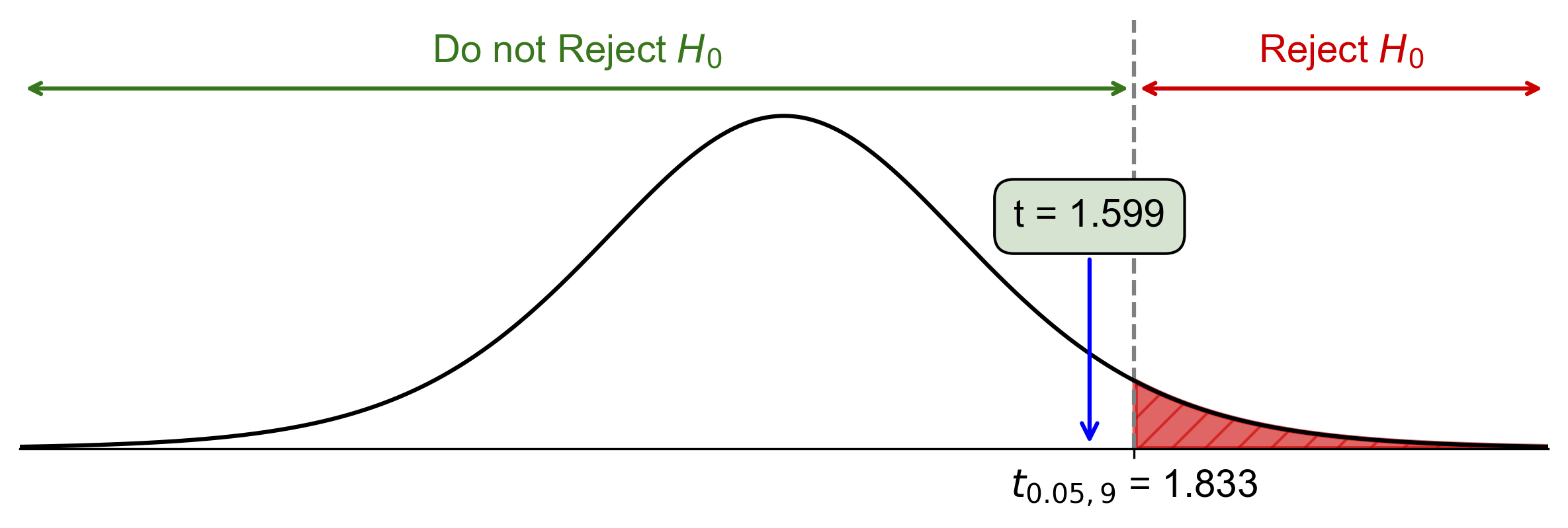
Fig. 7.46 Critical-value approach illustrating the rejection region and test statistic for Example 7.38.#
P-Value Approach:
Calculated P-Value: \(P(T > 1.599) \approx 0.0721\)
Since \(\text{P-value} = 0.0721 > \alpha = 0.05\), fail to reject \(H_0\).
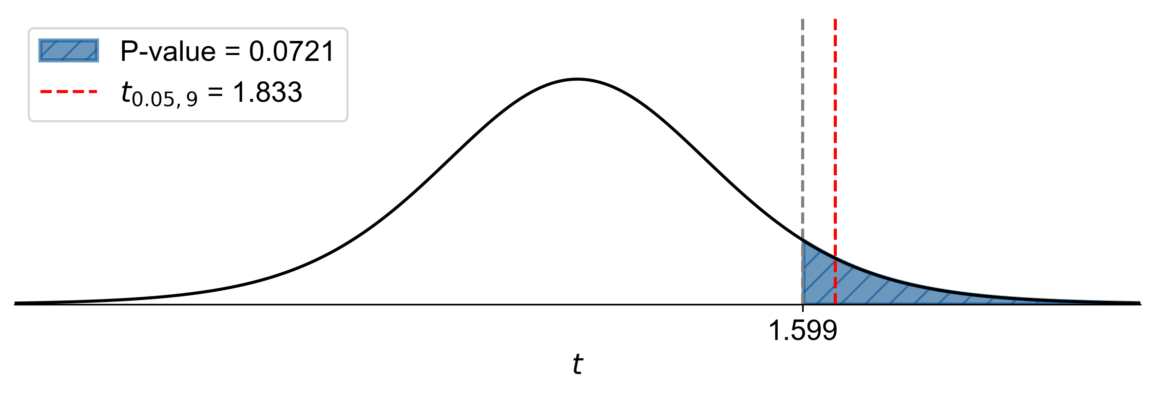
Fig. 7.47 P-value approach demonstrating the significance of the test statistic in relation to the null hypothesis for Example 7.38.#
Approximating P-Value Using the T-Distribution Table: We can also approximate the p-value using the t-distribution table for degrees of freedom (df = 9):
Area in One Tail
Critical t-Value (df = 9)
0.1
1.383
0.05
1.833
0.025
2.262
0.01
2.821
0.005
3.250
0.001
4.297
Given that our test statistic of 1.599 is between 1.383 and 1.833, we can infer that: 0.05 < P-value < 0.1.
Since \(\text{P-value} > \alpha = 0.05\), fail to reject \(H_0\).
Conclusion: At the 5% significance level, the data do not provide sufficient evidence to conclude that the mean test score for students using this teaching method is greater than 75%.
Example 7.39
A manufacturer claims that the average diameter of a batch of ball bearings is 50 mm. To verify this claim, a random sample of 16 ball bearings was measured, and the following diameters (in mm) were recorded:
At the 5% significance level, do the data provide sufficient evidence to conclude that the mean diameter of the ball bearings is different from 50 mm? Assume that the population standard deviation of the diameters is unknown.
Solution:
Hypothesis Test:
Null Hypothesis (\(H_0\)): \(\mu = 50\) mm
Alternative Hypothesis (\(H_a\)): \(\mu \neq 50\) mm
Sample Statistics:
\(n = 16\)
\(\overline{x} = 49.68\) mm (calculated as the mean of the sample data)
\(s = 1.267\) mm (sample standard deviation)
Significance Level: \(\alpha = 0.05\)
Test Statistic:
Degrees of Freedom: \(df = n - 1 = 15\)
Critical-Value Approach:
Critical value: \(t_{\alpha/2, df} = t_{0.025, 15} \approx \pm 2.131\)
Since \(\text{Test Statistic} = -1.006\) is within the range \(-2.131 < t < 2.131\), fail to reject \(H_0\).
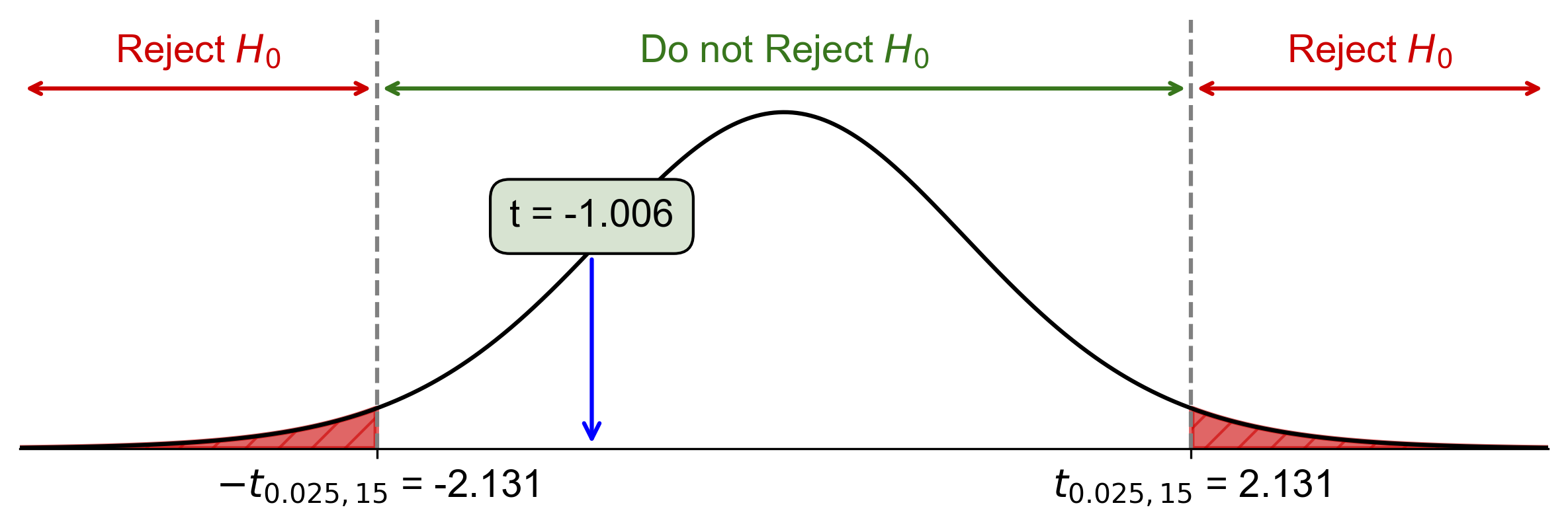
Fig. 7.48 Critical-value approach illustrating the rejection region and test statistic for Example 7.39.#
P-Value Approach:
Calculated P-Value: \(2 \times P(T < -1.006) \approx 0.3303\)
Since \(\text{P-value} = 0.3303 > \alpha = 0.05\), fail to reject \(H_0\).
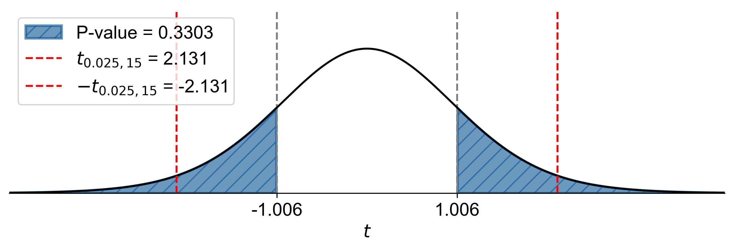
Fig. 7.49 P-value approach demonstrating the significance of the test statistic in relation to the null hypothesis for Example 7.39.#
Approximating P-Value Using the T-Distribution Table: We can also approximate the p-value using the t-distribution table for degrees of freedom (df = 15):
Area in One Tail
Critical t-Value (df = 15)
0.1
1.341
0.05
1.753
0.025
2.131
0.01
2.602
0.005
2.947
0.001
3.733
Given that our test statistic of |-1.006| = 1.006 is less than 1.341, we can infer that: The p-value (for a two-tailed test) is greater than 2 * 0.1 = 0.2.
Since \(\text{P-value} > 0.2 > \alpha = 0.05\), fail to reject \(H_0\).
Conclusion: At the 5% significance level, the data do not provide sufficient evidence to conclude that the mean diameter of the ball bearings is different from 50 mm.
Example 7.40
A researcher claims that the average height of a particular plant species is 15 cm. To test this claim, a random sample of 14 plants was measured, and the following heights (in cm) were recorded:
At the 5% significance level, do the data provide sufficient evidence to conclude that the mean height of this plant species is different from 15 cm? Assume that the population standard deviation of the heights is unknown.
Solution:
Hypothesis Test:
Null Hypothesis (\(H_0\)): \(\mu = 15\) cm
Alternative Hypothesis (\(H_a\)): \(\mu \neq 15\) cm
Sample Statistics:
\(n = 14\)
\(\overline{x} = 15.04\) cm (calculated as the mean of the sample data)
\(s = 0.237\) cm (sample standard deviation)
Significance Level: \(\alpha = 0.05\)
Test Statistic:
Degrees of Freedom: \(df = n - 1 = 13\)
Critical-Value Approach:
Critical value: \(t_{\alpha/2, df} = t_{0.025, 13} \approx \pm 2.160\)
Since \(\text{Test Statistic} = 0.563\) is within the range \(-2.160 < t < 2.160\), fail to reject \(H_0\).
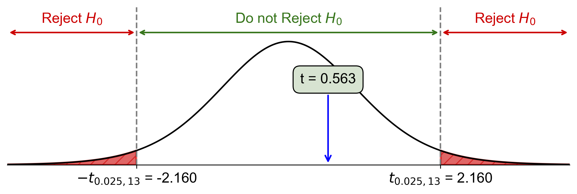
Fig. 7.50 Critical-value approach illustrating the rejection region and test statistic for Example 7.40.#
P-Value Approach:
Calculated P-Value: \(2 \times P(T > 0.563) \approx 0.5830\)
Since \(\text{P-value} = 0.5830 > \alpha = 0.05\), fail to reject \(H_0\).
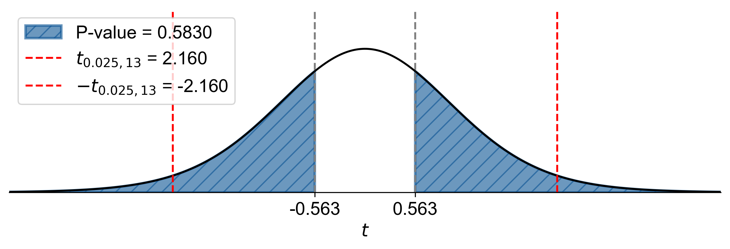
Fig. 7.51 P-value approach demonstrating the significance of the test statistic in relation to the null hypothesis for Example 7.40.#
Approximating P-Value Using the T-Distribution Table: We can also approximate the p-value using the t-distribution table for degrees of freedom (df = 13):
Area in One Tail
Critical t-Value (df = 13)
0.1
1.350
0.05
1.771
0.025
2.160
0.01
2.650
0.005
3.012
0.001
3.852
Given that our test statistic of 0.563 is less than 1.350, we can infer that: The p-value (for a two-tailed test) is greater than \(2 \times 0.1 = 0.2\).
Since \(\text{P-value} > 0.2 > \alpha = 0.05\), fail to reject \(H_0\).
Conclusion: At the 5% significance level, the data do not provide sufficient evidence to conclude that the mean height of this plant species is different from 15 cm.
