3.8. Law of Total Probability and Generalized form of Bayes’ Theorem#
3.8.1. Law of Total Probability#
The Law of Total Probability is a foundational rule in probability theory that relates the overall probability of an event, \(B\), to its constituent conditional probabilities. It provides a structured method to calculate the probability of \(B\) by considering all the distinct ways \(B\) can occur.
Here’s an enhanced explanation of the law [Devore et al., 2021]:
Mutually Exclusive Events: We define a collection of events, \(A_1, A_2, \ldots, A_n\), as mutually exclusive, meaning the occurrence of any one event excludes the possibility of any other event in this collection happening at the same time.
Exhaustive Events: These events are comprehensive, covering all possible outcomes of the experiment. In essence, it is guaranteed that one of the events \( A_1, A_2, \ldots, A_n \) must occur.
Event B: This is the event whose probability we wish to determine.
The law states that the probability of \(B\) is the sum of the probabilities of \(B\) occurring with each of the events \(A_i\):
This means that to find the probability of \(B\), we add together the probabilities of \(B\) happening alongside each of the mutually exclusive and exhaustive events \( A_i \).
An alternate formulation of the law uses conditional probabilities:
This expresses that the probability of \(B\) is the sum of the probabilities of \(B\) occurring given each event \( A_i \), multiplied by the probability of \(A_i \). This approach is utilized when we have knowledge of the conditional probabilities of \(B\) given \(A_i \) and the individual probabilities of \( A_i \).
Both expressions of the law serve to break down a complex probability into simpler, more calculable components. The Law of Total Probability is especially useful in scenarios where directly calculating \( P(B)\) is difficult, allowing us to use established probabilities to infer unknown ones. This law is a key element of probability theory, enhancing our grasp of the interconnections between individual probabilities within a larger probabilistic context.
Example 3.48
Customers who purchase a certain brand of laptop can choose among three different processor speeds. Of all laptops sold, 50% have the basic processor, 30% have the advanced processor, and 20% have the high-end processor. Of laptops with the basic processor, 5% experience a hardware failure within the first year, while 7% of those with the advanced processor and 9% of those with the high-end processor experience a failure. What is the probability that a randomly chosen laptop will experience a hardware failure within the first year?, the events are dependent. Adjust the probability for the second selection based on the outcome of the first.
Solution: Let’s denote the events as follows:
\( B \) = Laptop has a basic processor.
\( A \) = Laptop has an advanced processor.
\( H \) = Laptop has a high-end processor.
\( F \) = Laptop experiences a hardware failure within the first year.
Given:
\( P(B) = 0.50 \)
\( P(A) = 0.30 \)
\( P(H) = 0.20 \)
\( P(F|B) = 0.05 \)
\( P(F|A) = 0.07 \)
\( P(F|H) = 0.09 \)
We want to find \( P(F) \), the total probability of a laptop experiencing a hardware failure.
Using the Law of Total Probability:
Substituting the given probabilities:
Therefore, the probability that a randomly chosen laptop will experience a hardware failure within the first year is 6.4%.
Fig. 3.51 represents the decision-making process for purchasing a laptop with three different processor options: Basic Processor, Advanced Processor, and High-End Processor. Each processor option leads to two possible outcomes: Failure or No Failure, with associated probabilities. The probabilities of each outcome are multiplied by the initial decision probability to calculate the final outcome probabilities.
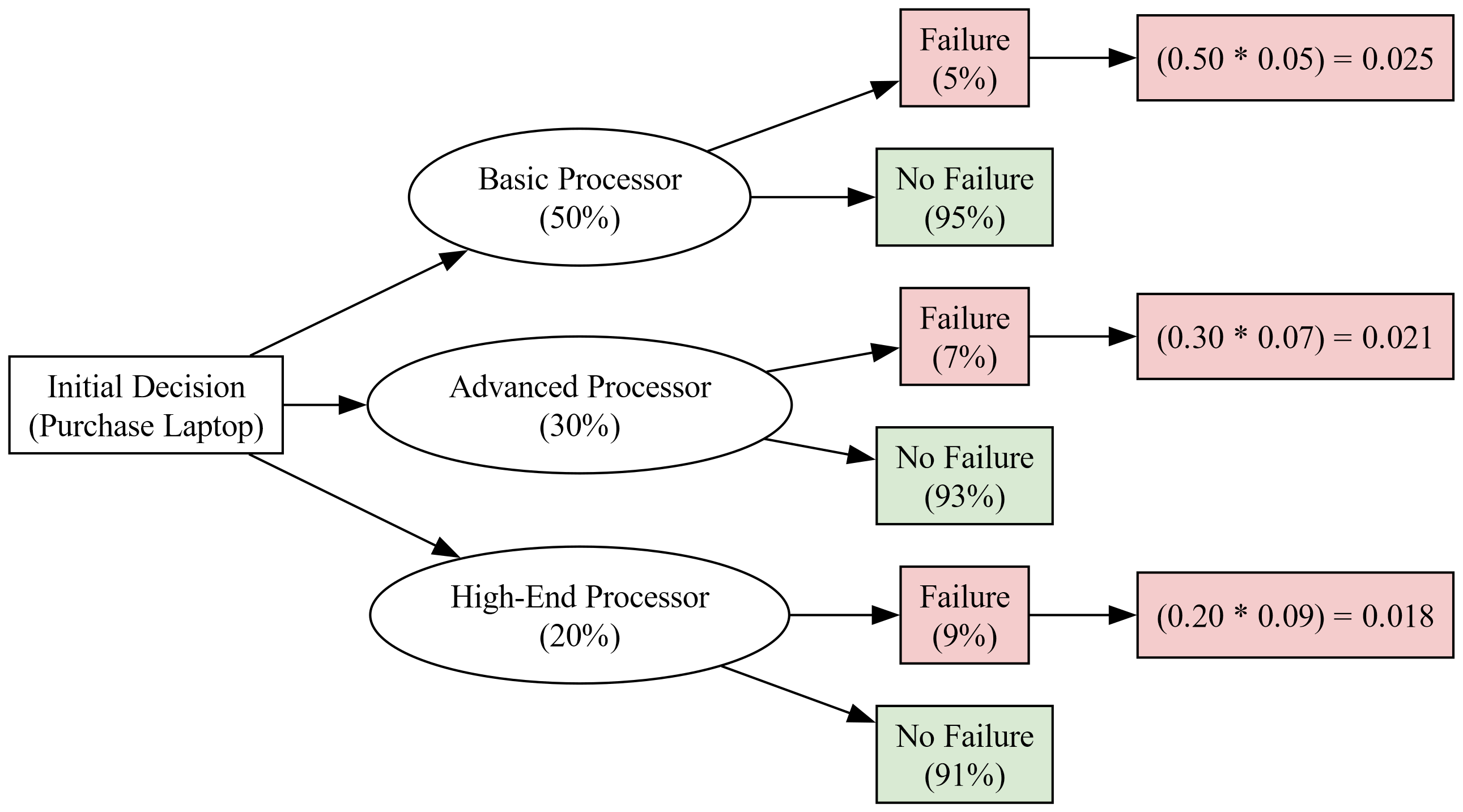
Fig. 3.51 Decision Analysis Flowchart for Laptop Purchase with Outcome Probabilities#
The sum of the failure probabilities across all processors gives us the total probability of failure: \( P(F) = 0.025 + 0.021 + 0.018 = 0.064 \) or 6.4%.
Example 3.49
A smartphone manufacturer offers three different battery sizes for their latest model. Of all smartphones sold, 40% have the standard battery, 35% have the extended battery, and 25% have the ultra-long-life battery. Of smartphones with the standard battery, 6% encounter battery issues within the first six months, while 4% of those with the extended battery and 2% of those with the ultra-long-life battery encounter issues. What is the probability that a randomly chosen smartphone will encounter battery issues within the first six months?
Solution: Let’s denote the events as follows:
\(S\) = Smartphone has a standard battery.
\(E\) = Smartphone has an extended battery.
\(U\) = Smartphone has an ultra-long-life battery.
\(I\) = Smartphone encounters battery issues within the first six months.
Given:
\(P(S) = 0.40\)
\(P(E) = 0.35\)
\(P(U) = 0.25\)
\(P(I|S) = 0.06\)
\(P(I|E) = 0.04\)
\(P(I|U) = 0.02\)
We want to find \( P(I) \), the total probability of a smartphone encountering battery issues.
Using the Law of Total Probability:
Substituting the given probabilities:
Therefore, the probability that a randomly chosen smartphone will encounter battery issues within the first six months is 4.3%.
Fig. 3.51 represents the decision-making process for purchasing a smartphone with three different battery options: Standard Battery, Extended Battery, and Ultra-Long-Life Battery. Each battery option leads to two possible outcomes: Battery Issues or No Issues, with associated probabilities. The probabilities of each outcome are multiplied by the initial decision probability to calculate the final outcome probabilities.
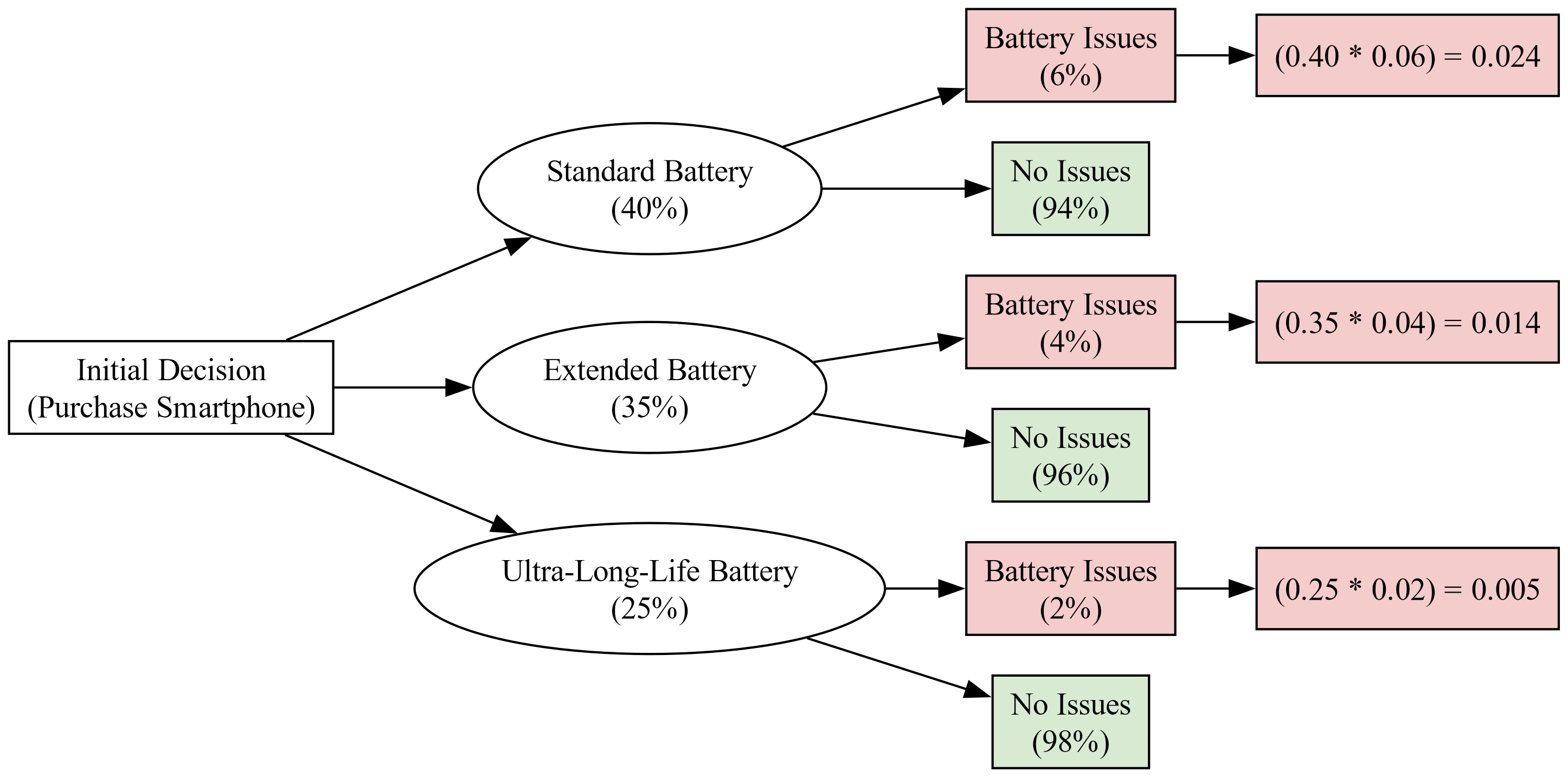
Fig. 3.52 Decision Analysis Flowchart for Smartphone Battery Issues with Outcome Probabilities#
3.8.2. Generalized form of Bayes’ Theorem#
The generalized form of Bayes’ Theorem allows us to update the probability of a hypothesis, \( H \), given evidence, \( E \), across multiple competing hypotheses. Here’s how it looks [Johnson et al., 2022]:
Where:
\(P(H_i|E)\) is the posterior probability of hypothesis \(H_i\) after observing evidence \(E\).
\(P(E|H_i)\) is the likelihood of observing evidence \(E\) given hypothesis \(H_i\).
\(P(H_i)\) is the prior probability of hypothesis \(H_i\).
The denominator, \(\sum_{j=1}^{n} P(E|H_j) \cdot P(H_j)\), is the normalizing constant, ensuring that the probabilities sum up to 1. It’s the sum of the products of the likelihood and the prior for all hypotheses.
This formula is used when you have more than two hypotheses and you want to find out the probability of one particular hypothesis being true given some evidence. It’s a powerful tool in statistical inference, allowing for the consideration of multiple scenarios and the updating of beliefs in light of new evidence.
Example 3.50
Imagine there are three diseases (\(D_1\), \(D_2\), \(D_3\)) that cause similar symptoms in patients. A medical test is designed to detect these diseases. The probabilities of the diseases in the general population and the effectiveness of the test are as follows:
Disease \(D_1\) occurs in 1% of the population.
Disease \(D_2\) occurs in 0.5% of the population.
Disease \(D_3\) occurs in 0.1% of the population.
The test has the following probabilities of correctly identifying a disease:
It correctly identifies \(D_1\) 99% of the time.
It correctly identifies \(D_2\) 95% of the time.
It correctly identifies \(D_3\) 90% of the time.
However, the test also has a 2% false positive rate for healthy individuals.
If a patient tests positive, what is the probability that they actually have each disease?
Solution: Let’s denote the events as follows:
\( H_i \) = Patient has disease \(D_i\).
\( E \) = Patient tests positive.
Given:
\(P(H_1) = 0.01\) (Disease \(D_1\))
\(P(H_2) = 0.005\) (Disease \(D_2\))
\(P(H_3) = 0.001\) (Disease \(D_3\))
\(P(E|H_1) = 0.99\) (Test correctly identifies \(D_1\))
\(P(E|H_2) = 0.95\) (Test correctly identifies \(D_2\))
\(P(E|H_3) = 0.90\) (Test correctly identifies \(D_3\))
\(P(E|H_0) = 0.02\) (False positive rate)
We want to find \( P(H_i|E) \) for \( i = 1, 2, 3 \).
First, we need to calculate \( P(E) \), the total probability of testing positive, which includes true positives and false positives:
Now, we apply the generalized Bayes’ Theorem to find the posterior probabilities:
For Disease \(D_1\):
For Disease \(D_2\):
For Disease \(D_3\):
So, if a patient tests positive, the probabilities that they actually have each disease are approximately:
28.1% for Disease \(D_1\)
13.5% for Disease \(D_2\)
2.6% for Disease \(D_3\)
Fig. 3.53 represents the decision-making process for diagnosing three diseases (\(D_1\), \(D_2\), \(D_3\)) based on a medical test. The probabilities of each disease in the general population and the effectiveness of the test are considered.
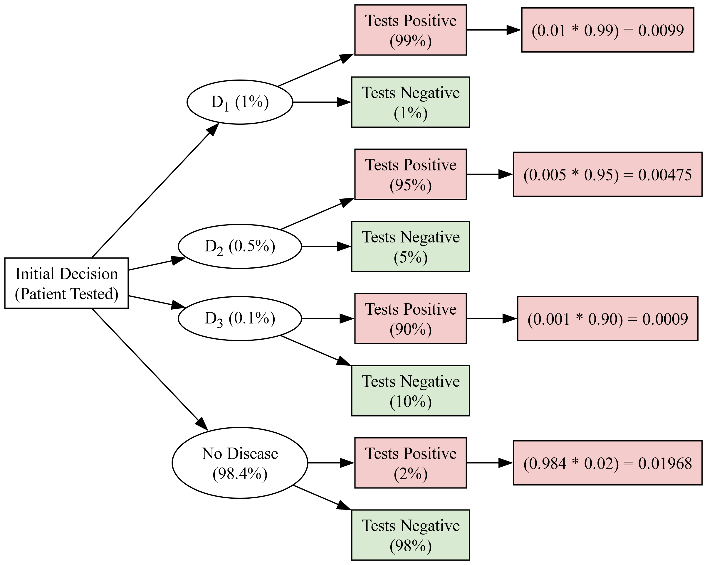
Fig. 3.53 Decision Analysis Flowchart for Disease Detection with Outcome Probabilities#
The sum of the probabilities of testing positive across all disease scenarios gives us the total probability of a positive test result: \(P(E) = 0.0099 + 0.00475 + 0.0009 + 0.01968 = 0.03523\).
Using the generalized Bayes’ Theorem, we find the posterior probabilities for each disease given a positive test result:
For Disease \(D_1\): \(P(H_1|E) = \dfrac{0.0099}{0.03523} \approx 0.281\)
For Disease \(D_2\): \(P(H_2|E) = \dfrac{0.00475}{0.03523} \approx 0.135\)
For Disease \(D_3\): \(P(H_3|E) = \dfrac{0.0009}{0.03523} \approx 0.026\)
So, if a patient tests positive, the probabilities that they actually have each disease are approximately:
28.1% for Disease \(D_1\)
13.5% for Disease \(D_2\)
2.6% for Disease \(D_3\)
Example 3.51
In a small town, there are three bakeries (Bakery A, Bakery B, and Bakery C) that supply bread to the local market. The market share of each bakery is known to be 50% for Bakery A, 30% for Bakery B, and 20% for Bakery C. It is also known that:
2% of the bread from Bakery A is stale.
1% of the bread from Bakery B is stale.
1.5% of the bread from Bakery C is stale.
A customer purchases a loaf of bread and finds it to be stale. What is the probability that the bread came from each bakery?
Solution: Let’s denote the events as follows:
\(H_A\) = Bread is from Bakery A.
\(H_B\) = Bread is from Bakery B.
\(H_C\) = Bread is from Bakery C.
\(S\) = Bread is stale.
Given:
\(P(H_A) = 0.50\)
\(P(H_B) = 0.30\)
\(P(H_C) = 0.20\)
\(P(S|H_A) = 0.02\)
\(P(S|H_B) = 0.01\)
\(P(S|H_C) = 0.015\)
We want to find \(P(H_i|S)\) for \(i = A, B, C\).
First, we calculate \(P(S)\), the total probability of getting a stale bread:
Now, we apply the generalized Bayes’ Theorem to find the posterior probabilities:
For Bakery A:
For Bakery B:
For Bakery C:
So, if a customer finds that their bread is stale, the probabilities that it came from each bakery are approximately:
62.5% for Bakery A
18.8% for Bakery B
18.8% for Bakery C
Fig. 3.54 represents the decision-making process for purchasing bread from three different bakeries (Bakery A, Bakery B, and Bakery C) and the probabilities of getting fresh or stale bread from each bakery.
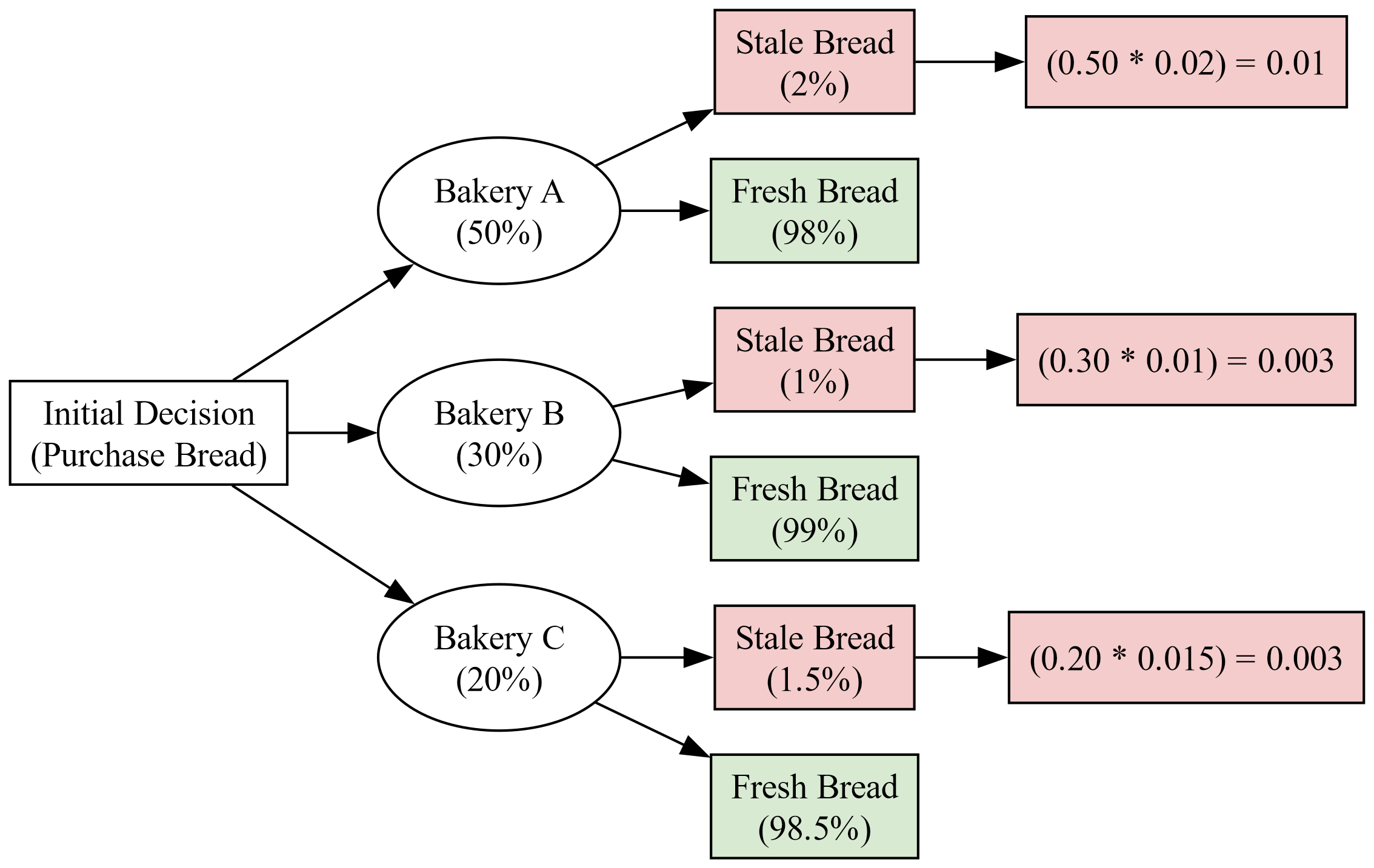
Fig. 3.54 Decision Analysis Flowchart for Bakery Bread Quality with Outcome Probabilities#
The sum of the probabilities of getting stale bread from each bakery gives us the total probability of a loaf being stale: \(P(S) = 0.01 + 0.003 + 0.003 = 0.016\) or 1.6%.
Using the generalized Bayes’ Theorem, we find the posterior probabilities for each bakery given that the bread is stale:
For Bakery A: \(P(H_A|S) = \dfrac{0.01}{0.016} \approx 0.625\) or 62.5%
For Bakery B: \(P(H_B|S) = \dfrac{0.003}{0.016} \approx 0.188\) or 18.8%
For Bakery C: \(P(H_C|S) = \dfrac{0.003}{0.016} \approx 0.188\) or 18.8%
So, if a customer finds that their bread is stale, the probabilities that it came from each bakery are approximately:
62.5% for Bakery A
18.8% for Bakery B
18.8% for Bakery C
