5.3. The Normal Distribution

5.3.1. Characteristics and Parameters of the Gaussian Curve

The normal distribution, also known as the Gaussian distribution or bell curve, is a continuous probability distribution that is symmetrical around its mean, denoted by \(\mu\). It is characterized by its mean and standard deviation, \(\sigma\), which determine the location and spread of the curve respectively.

• Mean (\(\mu\)): This is the average value where the peak of the bell curve is located. It represents the most probable value in the distribution.

• Standard Deviation (\(\sigma\)): This measures the amount of variation or dispersion from the mean. A smaller \(\sigma\) results in a steeper curve, while a larger \(\sigma\) leads to a wider and flatter curve.

When we encounter a quantity to be measured that follows a normal distribution with a specific mean (\(\mu\)) and standard deviation (\(\sigma\)), we denote this by writing:

(5.12)\[\begin{equation} X\sim N\left( \mu,\sigma \right) \quad\text{or}\quad X \sim N\left( \mu,\sigma^{2} \right) \end{equation}\]

In this notation, the symbol “~” signifies “follows” or “is distributed as”, “\(N\)” indicates the normal distribution, and (\(\mu\), \(\sigma\)) represents the specific mean and standard deviation values associated with the random variable \(X\).

Definition - The Normal Distribution

A continuous random variable is said to have a normal distribution when its distribution graph is symmetric and bell-shaped, as demonstrated in the accompanying figure.

If a continuous random variable has a distribution with a graph that is symmetric and bell-shaped, we say that it has a normal distribution.

(5.13)\[\begin{equation}f(x) = \frac{1}{\sigma \sqrt{2\pi}} e^{-\frac{1}{2} \left( \frac{x-\mu}{\sigma} \right)^2}\end{equation}\]

or

(5.14)\[\begin{equation}f\left( x \right) = \dfrac{1}{\sigma \sqrt{2 \pi}} \exp\left(- \dfrac{1}{2} \left( \dfrac{x - \mu}{\sigma} \right)^{2}\right)\end{equation}\]

5.3.2. Key Features of the Normal Distribution

The normal distribution, often depicted as a bell curve, is a cornerstone of probability and statistics. It underpins numerous real-world phenomena due to its unique characteristics:

1. Symmetry: The curve mirrors itself perfectly around the mean (\(\mu\)). This signifies that half the data falls above the mean and the other half below.

Fig. 5.13 illustrates the concept of symmetry in a normal distribution. The bell-shaped curve is perfectly symmetrical around the mean (\(\mu\)), which is the central vertical line. This symmetry indicates that the distribution of data is evenly balanced, with half of the data values falling above the mean and the other half below.

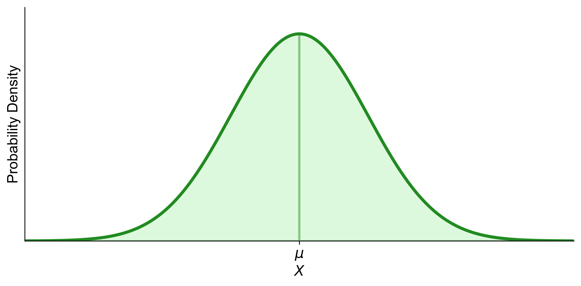
Fig. 5.13 Symmetry in Normal Distribution - A perfect balance around the mean (\(\mu\)), illustrating equal probabilities for data above and below this central value.

2. Central Tendency Harmony: The mean (\(\mu\)), median, and mode all coincide. In simpler terms, the center of the bell curve aligns with the average, the middle value, and the most frequent value in the data set.

Fig. 5.14 illustrates the concept of Central Tendency Harmony in a normal distribution. The bell-shaped curve is perfectly symmetrical around the mean (\(\mu\)), which is also the point where the median and mode coincide. This means that the center of the curve represents the average value (mean), the middle value (median), and the most frequent value (mode) in the data set. Fig. 5.14 also illustrates four different normal distributions, each represented by a bell-shaped curve with distinct mean (\(\mu\)) and standard deviation (\(\sigma\)) values.

• Pink Curve: This curve has a mean (\(\mu\)) of -2 and a standard deviation (\(\sigma\)) of 1. It is centered at -2 and has a moderate spread.

• Green Curve: This curve has a mean (\(\mu\)) of 0 and a standard deviation (\(\sigma\)) of 1/2. It is centered at 0 and is the steepest, indicating the least spread.

• Blue Curve: This curve has a mean (\(\mu\)) of 3 and a standard deviation (\(\sigma\)) of 2. It is centered at 3 and has the widest spread.

• Orange Curve: This curve has a mean (\(\mu\)) of 6 and a standard deviation (\(\sigma\)) of 1. It is centered at 6 and has a moderate spread.

• Purple Curve: This curve has a mean (\(\mu\)) of 8 and a standard deviation (\(\sigma\)) of 2/3. It is centered at 8 and has a moderate spread.

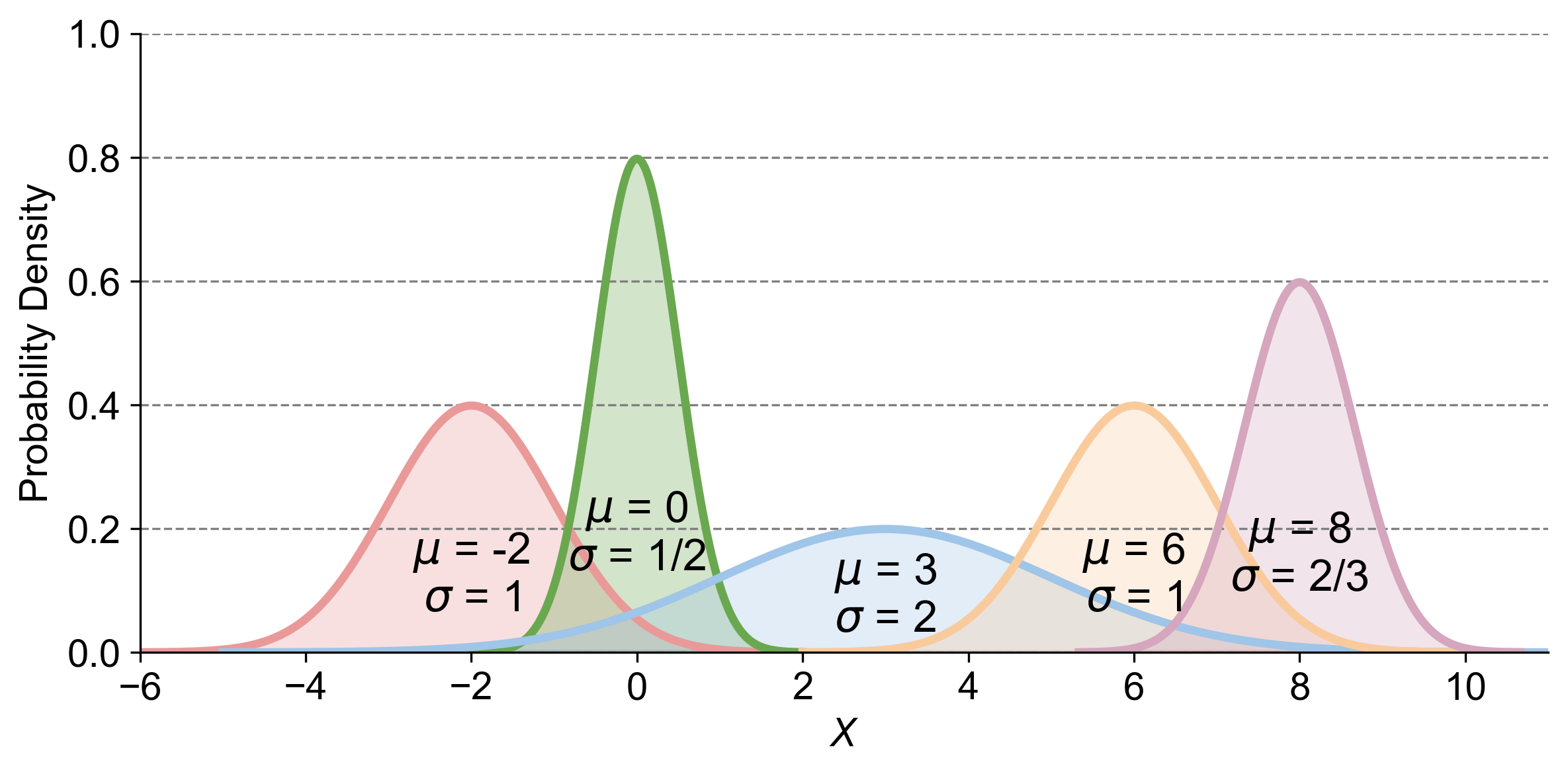
Fig. 5.14 Central Tendency Harmony in Normal Distribution - The mean (\(\mu\)), median, and mode all coincide at the peak of the bell curve, illustrating the balanced nature of the distribution.

3. Total Area Under the Curve: The entire area under the curve sums to one, reflecting the concept that the normal distribution represents probabilities.

Fig. 5.15 illustrates the concept of the total area under the curve in a normal distribution. The bell-shaped curve is symmetrical and peaks at the mean (\(\mu\)), which is indicated by a vertical dashed line. The area under the curve to the left of \(\mu\) is shaded and labeled “Area (Left Side) = 0.5,” while the area to the right is similarly shaded and labeled “Area (Right Side) = 0.5.” This shading demonstrates that each half of the curve represents a probability of 0.5, and together, they sum to a total probability of 1.

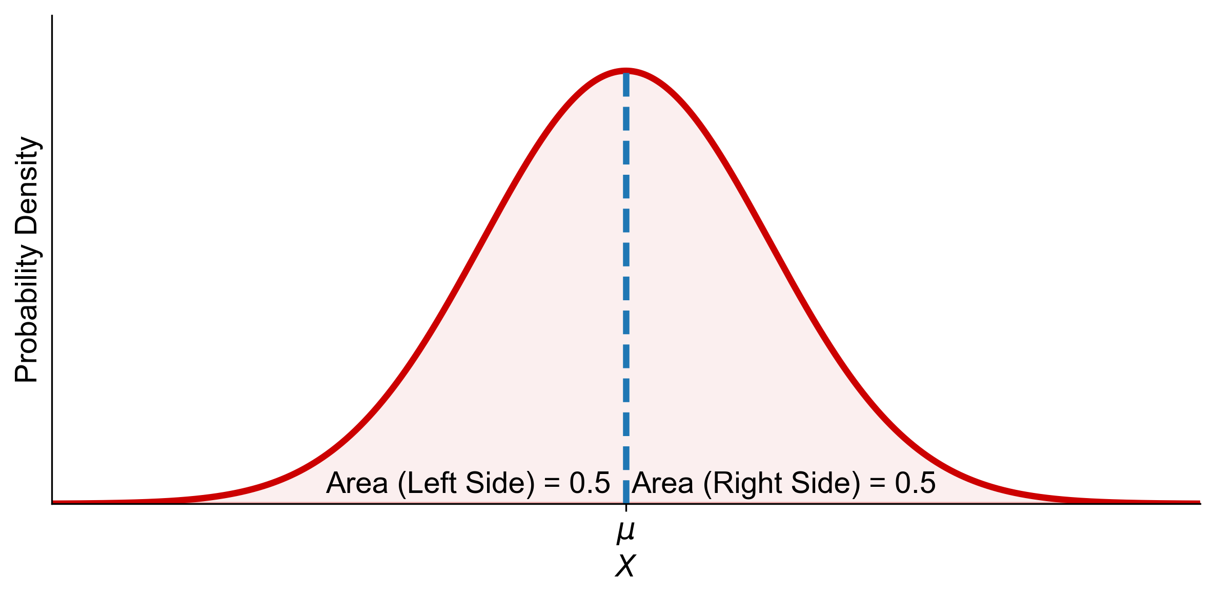
Fig. 5.15 Total Area Under the Curve in Normal Distribution - The entire area sums to one, illustrating that the normal distribution represents probabilities.

5.3.3. The Empirical Rule and the Normal Distribution

The Empirical Rule, also known as the 68-95-99.7 Rule, is a statistical guideline that describes how data in a normal distribution tends to behave relative to the mean (average):

• Within One Standard Deviation (\(\sigma\)): About 68% of the data points are found within one standard deviation from the mean. This range is the most densely populated area of the curve, indicating where data points are most likely to occur.

Fig. 5.16 illustrates the Empirical Rule, also known as the 68-95-99.7 Rule, for a normal distribution. The bell-shaped curve is centered around the mean (\(\mu\)), with the x-axis labeled in terms of standard deviations (\(\sigma\)) from the mean: \(\mu-3\sigma\), \(\mu-2\sigma\), \(\mu-\sigma\), \(\mu\), \(\mu+\sigma\), \(\mu+2\sigma\), and \(\mu+3\sigma\). The y-axis is labeled ‘Probability Density.’ The area under the curve between \(\mu-\sigma\) and \(\mu+\sigma\) is shaded, representing “Almost 68% of data.” This shaded area highlights that approximately 68% of data points in a normal distribution fall within one standard deviation of the mean, which is the most densely populated region of the curve.

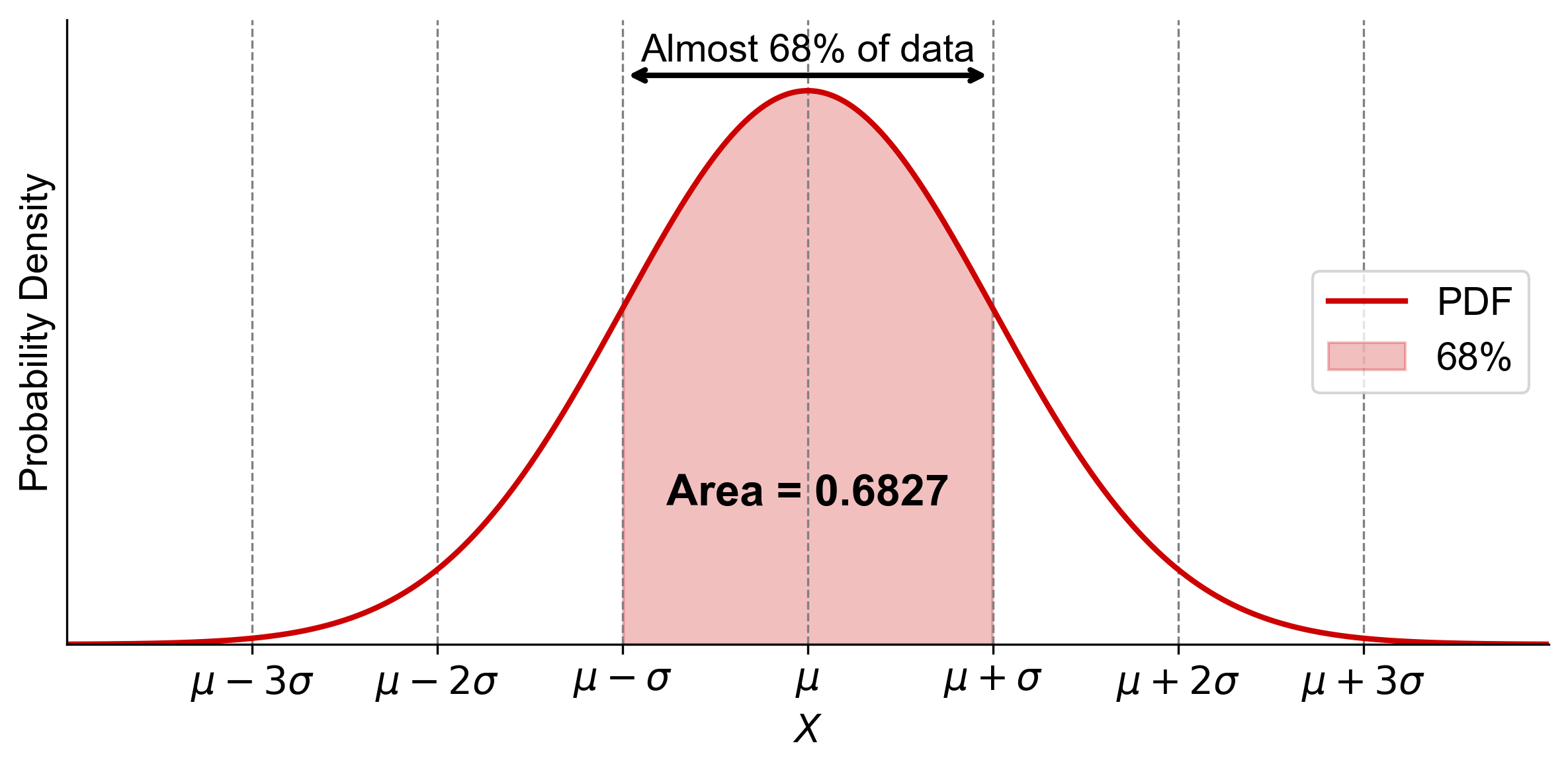
Fig. 5.16 Illustration of the Empirical Rule showing that approximately 68% of data in a normal distribution falls within one standard deviation (\(\sigma\)) of the mean (\(\mu\)).

• Within Two Standard Deviations (\(2\sigma\)): Expanding the range to two standard deviations from the mean captures approximately 95% of the data. This wider band encompasses the vast majority of occurrences, leaving only 5% in the tails.

Fig. 5.17 illustrates the Empirical Rule, also known as the 68-95-99.7 Rule, for a normal distribution. The bell-shaped curve is centered around the mean (\(\mu\)), with the x-axis labeled in terms of standard deviations (\(\sigma\)) from the mean: \(\mu-3\sigma\), \(\mu-2\sigma\), \(\mu-\sigma\), \(\mu\), \(\mu+\sigma\), \(\mu+2\sigma\), and \(\mu+3\sigma\). The y-axis is labeled ‘Probability Density.’ The area under the curve between \(\mu-2\sigma\) and \(\mu+2\sigma\) is shaded, representing “Almost 95% of data.” This shaded area highlights that approximately 95% of data points in a normal distribution fall within two standard deviations of the mean, which is a significant portion of the data.

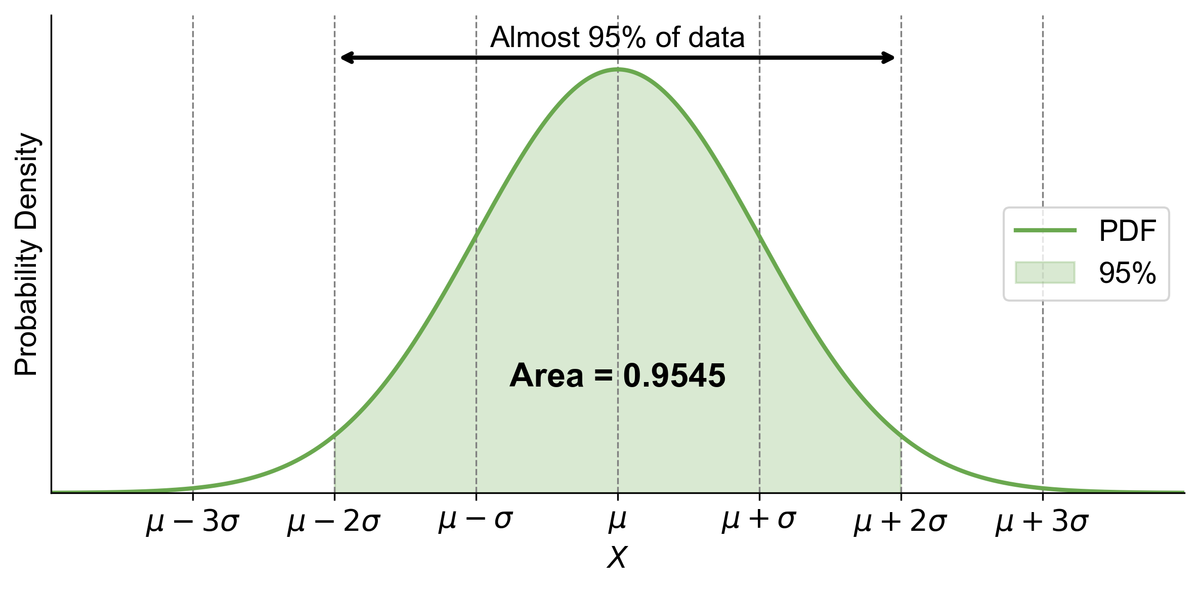
Fig. 5.17 Illustration of the Empirical Rule showing that approximately 95% of data in a normal distribution falls within two standard deviations (\(\sigma\)) of the mean (\(\mu\)).

• Within Three Standard Deviations (\(3\sigma\)): Extending to three standard deviations includes about 99.7% of the data. This almost complete coverage of the data points illustrates the rarity of values falling outside this range.

Fig. 5.18 illustrates the Empirical Rule, also known as the 68-95-99.7 Rule, for a normal distribution. The bell-shaped curve is centered around the mean (\(\mu\)), with the x-axis labeled in terms of standard deviations (\(\sigma\)) from the mean: \(\mu-3\sigma\), \(\mu-2\sigma\), \(\mu-\sigma\), \(\mu\), \(\mu+\sigma\), \(\mu+2\sigma\), and \(\mu+3\sigma\). The y-axis is labeled ‘Probability Density.’ The area under the curve between \(\mu-3\sigma\) and \(\mu+3\sigma\) is shaded, representing “Almost 99.7% of data.” This shaded area highlights that approximately 99.7% of data points in a normal distribution fall within three standard deviations of the mean, covering nearly all the data.

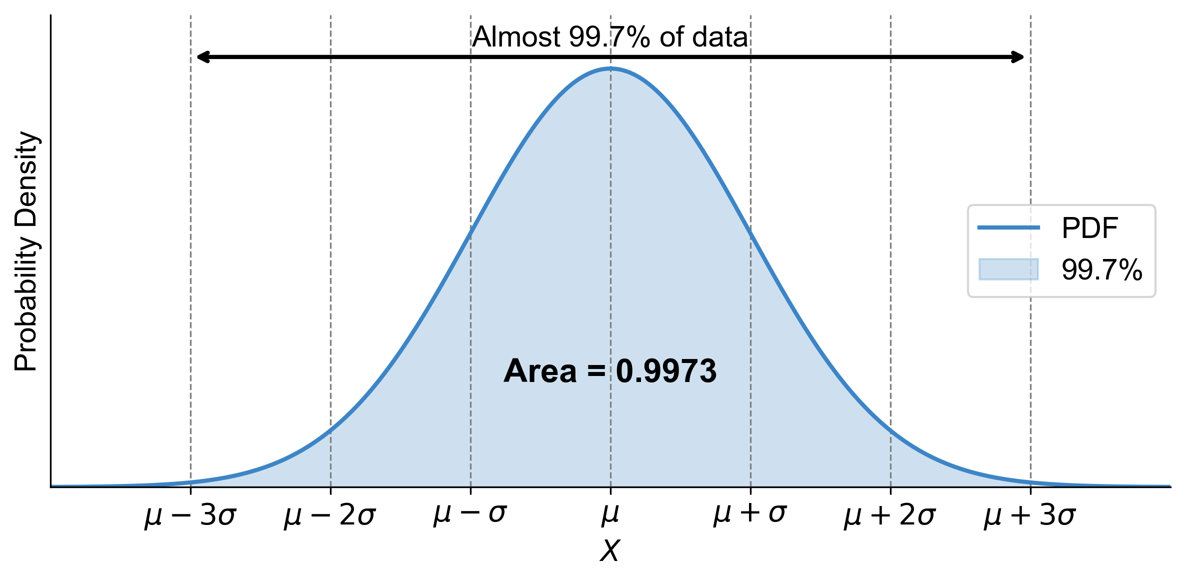
Fig. 5.18 Illustration of the Empirical Rule showing that approximately 99.7% of data in a normal distribution falls within three standard deviations (\(\sigma\)) of the mean (\(\mu\)).

In summary, the Empirical Rule states that 68%, 95%, and 99.7% of data fall within one, two, and three standard deviations (\(\sigma\)) from the mean (\(\mu\)), respectively, illustrating how data points are distributed around the central value.

Fig. 5.19 provides a comprehensive summary of the Empirical Rule, also known as the 68-95-99.7 Rule, for a normal distribution. The areas under the curve are shaded to represent different percentages of data within standard deviations from the mean:

• 68% of data: Within \(\mu\) ± \(\sigma\)

• 95% of data: Within \(\mu\) ± 2\(\sigma\)

• 99.7% of data: Within \(\mu\) ± 3\(\sigma\)

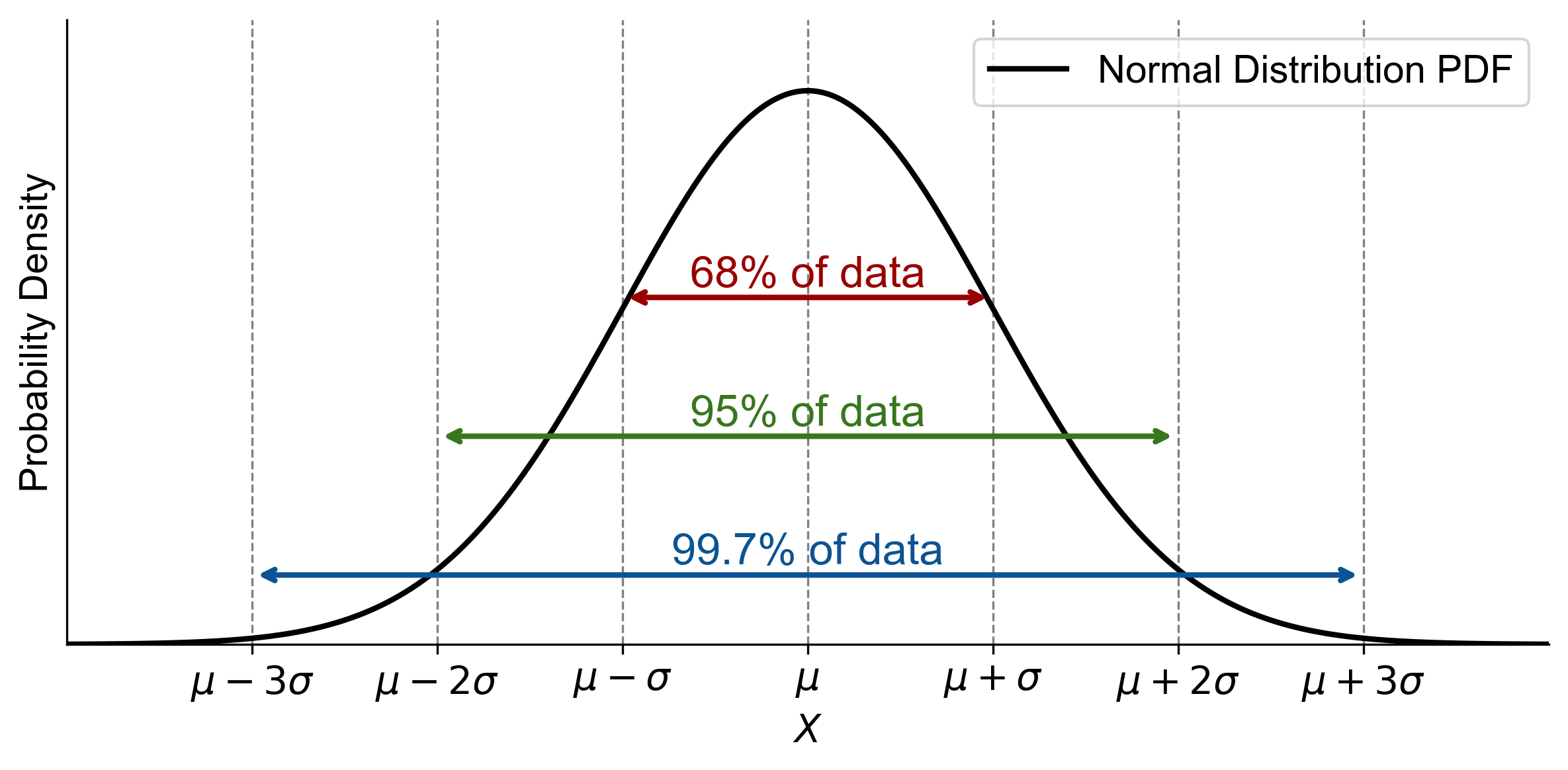
Fig. 5.19 Summary of the Empirical Rule showing that approximately 68%, 95%, and 99.7% of data in a normal distribution fall within one, two, and three standard deviations (\(\sigma\)) of the mean (\(\mu\)), respectively.