5.7. The Central Limit Theorem#
The Central Limit Theorem (CLT) is often referred to as the ‘great equalizer’ in the realm of statistics due to its powerful implications. It is a cornerstone concept that supports the practice of using sample means to estimate the means of entire populations. The theorem’s key assertion is that the distribution of sample means will approximate a normal distribution, commonly known as a bell curve, as the size of the sample grows larger. This holds true regardless of the shape of the population’s distribution.
In mathematical terms, if we consider a random variable \(X\), which has a mean of \(\mu_X\) and a standard deviation of \(\sigma_X\), the theorem states that the distribution of the sample means \(\bar{X}\) will approach a normal distribution with the same mean \(\mu_X\) and a standard deviation of \(\frac{\sigma_X}{\sqrt{n}}\), where \(n\) is the sample size. This is expressed by the formula:
The practical implication of the CLT is significant: it enables us to use the normal distribution model to draw conclusions about the population mean, even when the population itself does not follow a normal distribution. This is particularly useful because the normal distribution has well-known properties that allow for easier calculation of probabilities and confidence intervals.
Example 5.33
Imagine we’re interested in the average height of adult males in a city. The population distribution of heights may not be normal; it could be skewed or have multiple peaks. However, if we take multiple random samples of, say, 30 men each and calculate the average height for each sample, the distribution of these sample averages will tend to look more like a normal distribution. As the sample size increases, this approximation improves. If the true average height is 175 cm with a standard deviation of 10 cm, the distribution of the sample means for samples of size 30 will be approximately normal with a mean of 175 cm and a standard deviation of \(\frac{10}{\sqrt{30}}\) cm. This allows us to make predictions about the average height of all adult males in the city based on our sample data.
The Central Limit Theorem (CLT) serves as a foundational principle in statistics, enabling us to make inferences about population parameters using sample statistics. It assures us that for a sufficiently large sample size, the distribution of the sample mean \(\overline{x}\) will approximate a normal distribution, irrespective of the original distribution of the variable. This approximation improves as the sample size increases.
Key Points:
If the original variable follows a normal distribution, the sample means will also be normally distributed, and this is true for any sample size \(n\).
For non-normally distributed variables, a sample size of 30 or more is generally considered sufficient for the sample means to approximate a normal distribution. The larger the sample size, the closer the approximation to a normal distribution.
Standardization Formula: When standardizing the sample mean to compare it to a normal distribution, we use the following formula:
Where \(Z\) is the standard normal variable, \(\overline{x}\) is the sample mean, \(\mu\) is the population mean, \(\sigma\) is the population standard deviation, and \(n\) is the sample size.
Table 5.4 summarizes the conditions under which the CLT applies and the corresponding standardization formula:
Distribution of the Parent Population |
Sample Size |
Sampling Distribution of the Sample Mean |
Shape of the Sampling Distribution |
Standardization Formula |
|---|---|---|---|---|
Normal or Approximately Normal |
Any \(n\) |
\(\overline{x} \sim N(\mu, \sigma/\sqrt{n})\) |
Normal |
\(Z = \dfrac{(\overline{x} - \mu)}{\sigma/\sqrt{n}}\) |
Unknown / Non-normal |
\(n \geq 30\) |
Approximates Normal |
Approximates Normal |
\(Z = \dfrac{(\overline{x} - \mu)}{\sigma/\sqrt{n}}\) |
Example 5.34
Let’s consider an example where we’re studying the average weight of pumpkins in a large farm. The distribution of weights is unknown and potentially non-normal. By taking a sample of 50 pumpkins and calculating the average weight, we can apply the CLT to conclude that this sample mean will approximate a normal distribution. If the average weight of the sample is 10 kg with a standard deviation of 2 kg, we can standardize this sample mean to compare it to a normal distribution using the formula above.
5.7.1. The Central Limit Theorem and the Sampling Distribution of \(\bar{x}\)#
When we draw samples of size \(n\) from a population with a mean \(\mu\) and standard deviation \(\sigma\), the sample mean \(\overline{x}\) has its own distribution with the following properties:
The mean of \(\overline{x}\), denoted as \(\mu_{\overline{x}}\), is equal to the population mean \(\mu\).
The standard deviation of \(\overline{x}\), denoted as \(\sigma_{\overline{x}}\), is the population standard deviation \(\sigma\) divided by the square root of the sample size \(n\), which is also known as the standard error of the mean (SEM).
These relationships are expressed mathematically as:
Key Observations:
If the population variable \(x\) is normally distributed, the distribution of \(\overline{x}\) will also be normal for any sample size.
For large sample sizes, \(\overline{x}\) will be approximately normally distributed, regardless of the population distribution of \(x\).
Fig. 5.63 presents a 3x3 grid of panels, each showing histograms overlaid with kernel density estimates (KDEs) to illustrate the sampling distribution of the sample mean for different sample sizes (\(n = 10\), \(n = 20\), \(n = 30\)) and different population distributions (Normal in blue, Exponential in green, Uniform in red). Explanation:
Top Row (Normal Population):
\(n = 10\), \(20\), \(30\): As sample size increases, the sampling distribution of the sample mean becomes more normally distributed, demonstrating the Central Limit Theorem (CLT).
Middle Row (Exponential Population):
\(n = 10\), \(20\), \(30\): The sampling distributions show increasing normality with larger sample sizes, illustrating the CLT’s robustness across different population distributions.
Bottom Row (Uniform Population):
\(n = 10\), \(20\), \(30\): Similar to the other rows, the sampling distributions become more normally distributed with larger sample sizes, highlighting the CLT’s principle that larger sample sizes lead to normality regardless of the original population distribution.
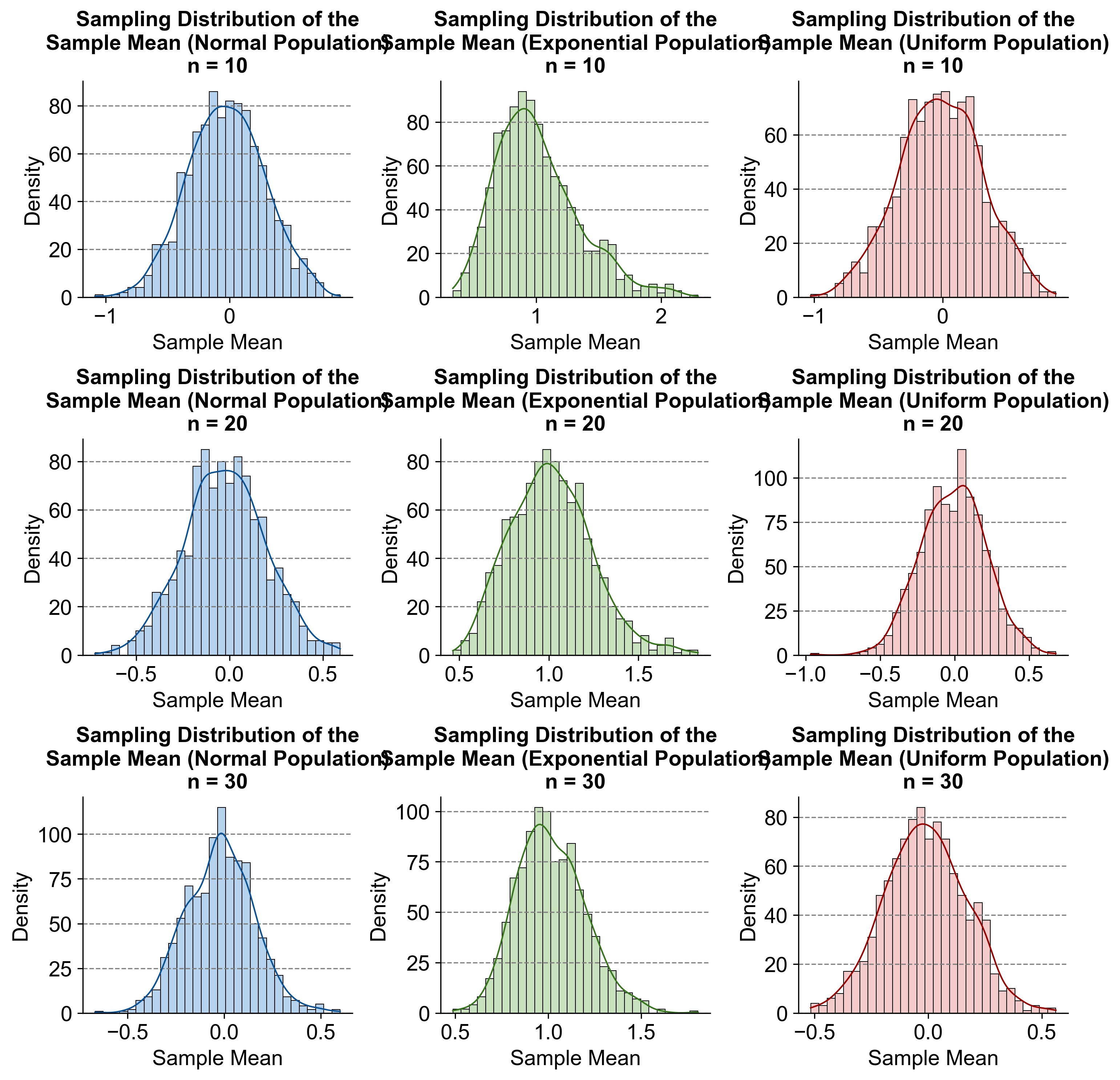
Fig. 5.63 Sampling Distribution of the Sample Mean for Different Sample Sizes and Population Distributions.#
Remark
As the sample size \(n\) increases, the standard deviation of the distribution of sample means, known as the standard error, decreases.
For samples of size \(n\), the standard error of the sample mean \(\bar{X}\) is equal to the population standard deviation \(\sigma\) divided by the square root of the sample size. Mathematically, this relationship is expressed as:
This equation illustrates that the standard deviation of all possible sample means (standard error) is inversely proportional to the square root of the sample size \(n\). Consequently, as the sample size increases, the standard error decreases, leading to a more precise estimate of the population mean.
Example 5.35
Consider the sediment density (in grams per cubic centimeter, \(g/cm^3\)) of a randomly selected specimen from a specific region. This density is assumed to be normally distributed with a mean (\(\mu\)) of \(2.65~g/cm^3\) and a standard deviation (\(\sigma\)) of \(0.85~g/cm^3\), as suggested in the study “Modeling Sediment and Water Column Interactions for Hydrophobic Pollutants,” published in Water Research in 1984.
a) If a random sample of 25 specimens is selected, what is the probability that the sample average sediment density is at most \(3.00~g/cm^3\)?
b) If a random sample of 25 specimens is selected, what is the probability that the sample average sediment density is between \(2.65~g/cm^3\) and \(3.00~g/cm^3\)?
Solution:
Given:
Population mean (\(\mu\)) = \(2.65~g/cm^3\)
Population standard deviation (\(\sigma\)) = \(0.85~g/cm^3\)
Sample size (\(n\)) = \(25\)
The distribution of the sample mean \(\bar{X}\) follows a normal distribution with:
Mean:
Standard deviation:
We can standardize our sample mean to find the z-score:
a) For \(\bar{x} = 3.00~g/cm^3\):
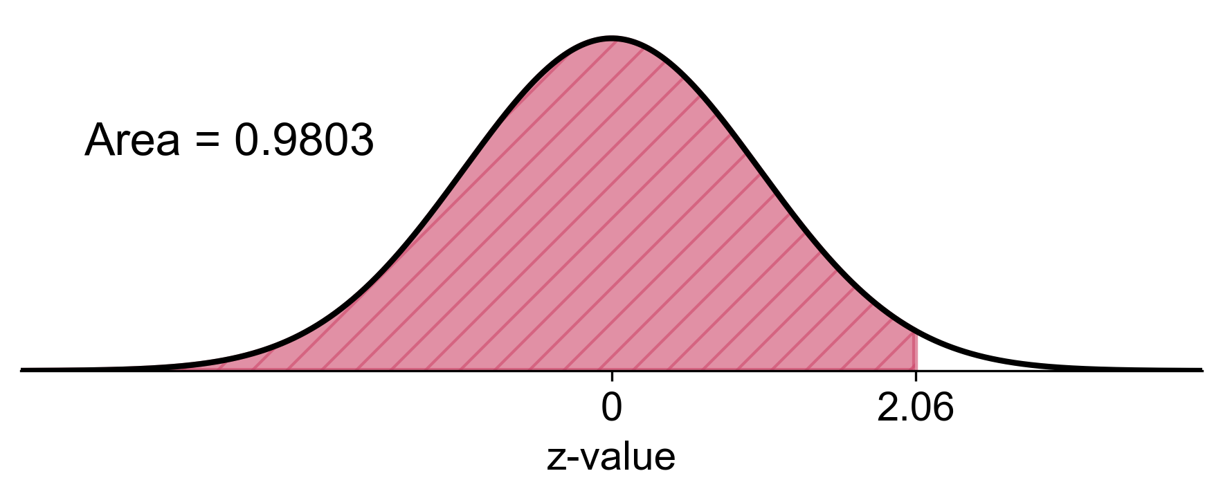
Fig. 5.64 Probability that the sample average sediment density is at most \(3.00~g/cm^3\).#
b) We need to find \(P(2.65 \leq \bar{X} \leq 3.00)\):
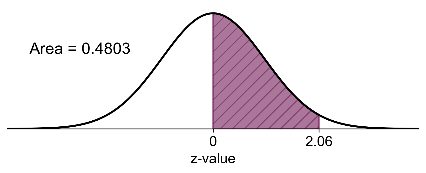
Fig. 5.65 Probability that the sample average sediment density is between \(2.65~g/cm^3\) and \(3.00~g/cm^3\).#
Example 5.36
The uric acid levels in normal adult males are approximately normally distributed with a mean (\(\mu\)) of 5.7 mg and a standard deviation (\(\sigma\)) of 1 mg. We are interested in finding the probability that a sample of size \(n = 9\) will yield a sample mean (\(\bar{X}\)) in certain ranges.
a) Find the probability that the sample mean is greater than 6 mg.
b) Find the probability that the sample mean is between 5 mg and 6 mg.
c) Find the probability that the sample mean is less than 5.2 mg.
Solution: First, let’s calculate the standard error of the sampling distribution:
a) To find the probability that the sample mean is greater than 6 mg:
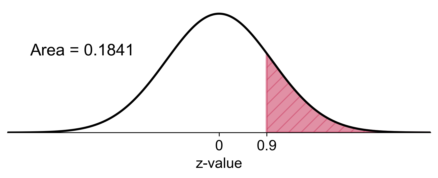
Fig. 5.66 Probability of sample mean greater than 6 mg in the sampling distribution#
b) To find the probability that the sample mean is between 5 mg and 6 mg:
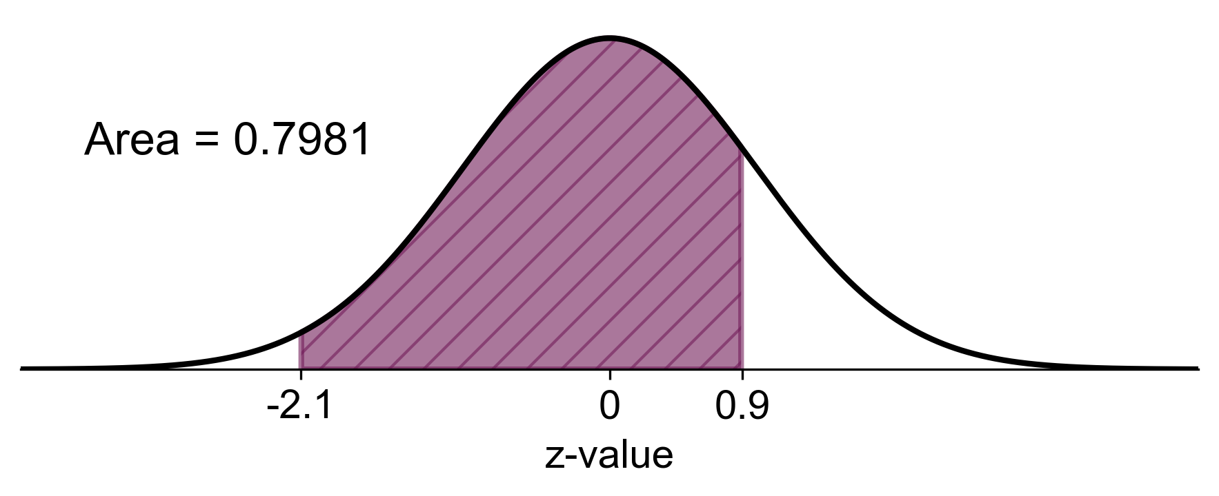
Fig. 5.67 Probability of sample mean between 5 mg and 6 mg in the sampling distribution#
c) To find the probability that the sample mean is less than 5.2 mg:
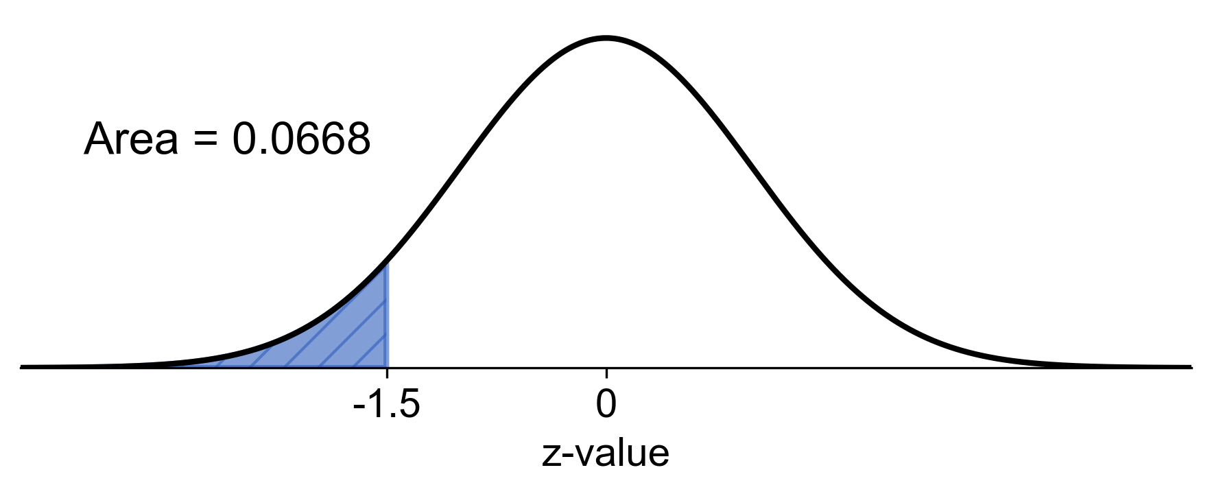
Fig. 5.68 Probability of sample mean less than 5.2 mg in the sampling distribution#
Example 5.37
The uric acid levels in normal adult males are approximately normally distributed with a mean (\(\mu\)) of 5.7 mg and a standard deviation (\(\sigma\)) of 1 mg. For a sample of size \(n = 9\), calculate:
a) The probability that the sample mean (\(\bar{X}\)) is greater than 6 mg.
b) The probability that the sample mean (\(\bar{X}\)) is between 5.5 mg and 6 mg.
Solution: We will apply the Central Limit Theorem. The sampling distribution of the mean for samples of size \(n = 9\) will be normally distributed with:
Mean: \(\mu_{\bar{X}} = \mu = 5.7\) mg
Standard error: \(\sigma_{\bar{X}} = \frac{\sigma}{\sqrt{n}} = \frac{1}{\sqrt{9}} = \frac{1}{3}\) mg
Let’s calculate the probabilities:
a) Probability that the sample mean is greater than 6 mg:
Using a standard normal table or calculator:
Therefore, there’s approximately an 18.41% chance that a sample of 9 males will have a mean uric acid level greater than 6 mg.
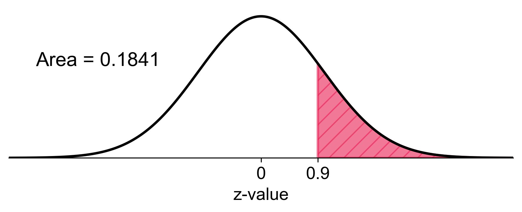
Fig. 5.69 Probability of sample mean greater than 6 mg in the sampling distribution#
b) Probability that the sample mean is between 5.5 mg and 6 mg:
Therefore, there’s approximately a 54.16% chance that a sample of 9 males will have a mean uric acid level between 5.5 mg and 6 mg.
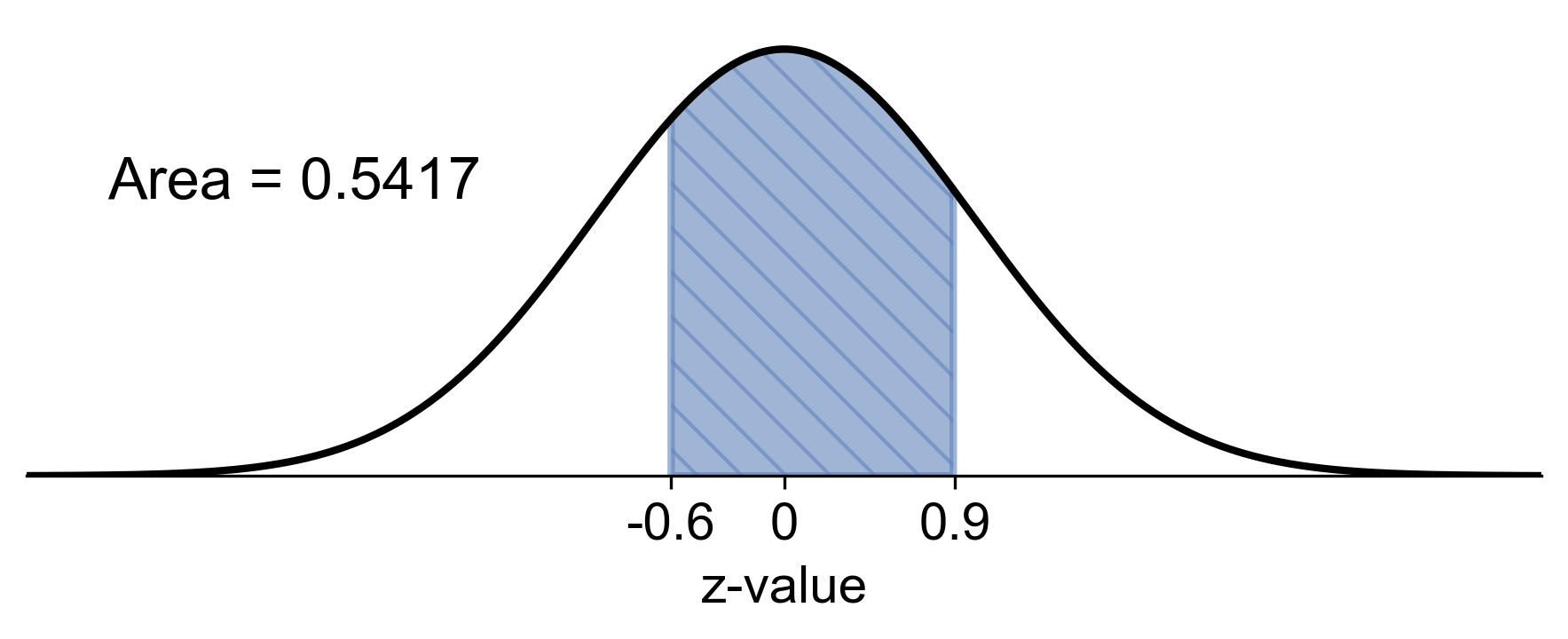
Fig. 5.70 Probability of sample mean between 5.5 mg and 6 mg in the sampling distribution#
Example 5.38
Cholesterol levels in adults are normally distributed with a mean (\(\mu\)) of 200 mg/dL and a standard deviation (\(\sigma\)) of 30 mg/dL. Given a sample of 40 adults, determine the probability that their average cholesterol level exceeds 210 mg/dL.
Solution: We will apply the Central Limit Theorem to calculate the probability concerning the sample mean.
First, let’s identify the key information:
Population mean: \(\mu = 200\) mg/dL
Population standard deviation: \(\sigma = 30\) mg/dL
Sample size: \(n = 40\)
We’re looking for \(P(\bar{X} > 210)\)
The sampling distribution of the mean will be normally distributed with:
Mean: \(\mu_{\bar{X}} = \mu = 200\) mg/dL
Standard error: \(\sigma_{\bar{X}} = \frac{\sigma}{\sqrt{n}} = \frac{30}{\sqrt{40}} = 4.74\) mg/dL
Now, let’s calculate the z-score for the sample mean of 210 mg/dL:
We want to find \(P(\bar{X} > 210)\), which is equivalent to \(P(Z > 2.11)\).
Using the standard normal distribution table or a calculator:
Therefore, there is approximately a 1.74% chance that the sample mean cholesterol level of 40 adults will exceed 210 mg/dL.
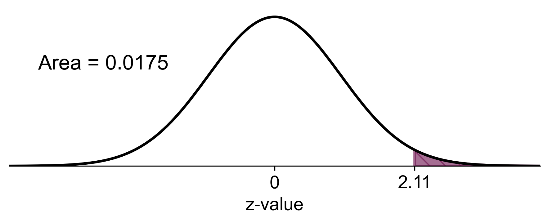
Fig. 5.71 Probability of sample mean cholesterol level exceeding 210 mg/dL in the sampling distribution#
This figure illustrates the sampling distribution of the mean cholesterol levels. The shaded area represents the probability that the sample mean exceeds 210 mg/dL.
Example 5.39
The heights of men in a certain population are normally distributed with a mean (\(\mu\)) of 69.7 inches and a standard deviation (\(\sigma\)) of 3.1 inches.
a) What is the probability that a randomly selected man from this population will be less than 72 inches tall?
b) If a random sample of 25 men is selected, what is the probability that their average height will be between 68.7 inches and 70.7 inches?
Solution:
a) To find the probability that a man is less than 72 inches tall, we calculate the z-score and refer to the standard normal distribution:
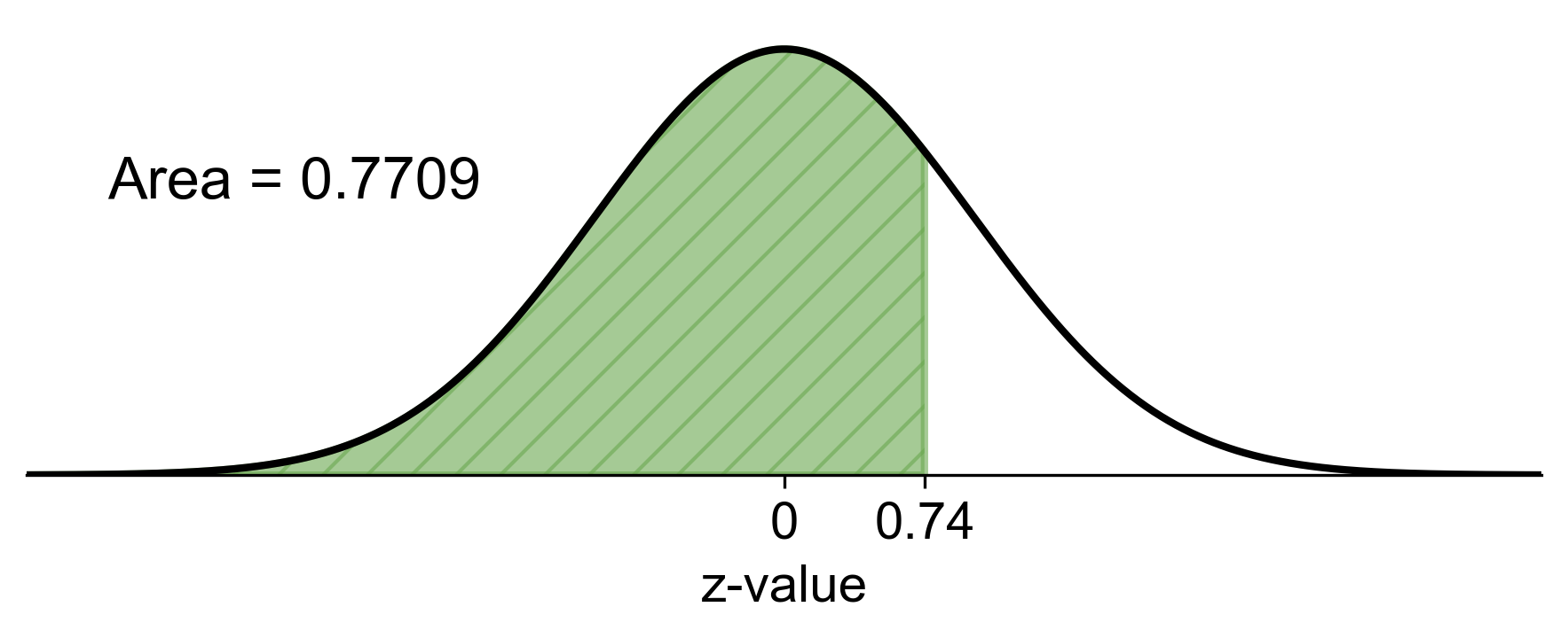
Fig. 5.72 Probability that a randomly selected man is less than 72 inches tall#
b) For the sample of 25 men, we calculate the z-scores for the mean heights of 68.7 inches and 70.7 inches and find the cumulative probability:
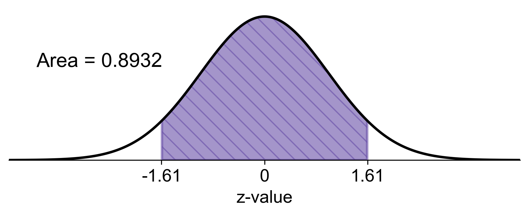
Fig. 5.73 Probability that the average height of 25 men is between 68.7 inches and 70.7 inches#
This means:
a) There is a 77.09% chance that a randomly selected man will be less than 72 inches tall.
b) There is an 89.32% chance that the average height of a sample of 25 men will be between 68.7 inches and 70.7 inches.
Certainly! I’ll add the figures to the solution as requested. Here’s the updated version:
Example 5.40
In a health examination survey of a particular province in Canada, the fasting blood glucose levels are normally distributed with a mean (\(\mu\)) of 99.0 mg/dL and a standard deviation (\(\sigma\)) of 12 mg/dL.
a) What is the probability that a randomly selected individual will have a blood sugar reading greater than 120 mg/dL?
b) If a random sample of 36 individuals is selected, what is the probability that their average blood sugar reading is between 96 and 102 mg/dL?
Solution: The blood glucose levels follow a normal distribution: \(X \sim N(\mu = 99.0, \sigma = 12)\).
a) To find the probability of a blood sugar reading greater than 120 mg/dL, we calculate the z-score:
Using the standard normal distribution, we find the probability associated with \(Z > 1.75\).
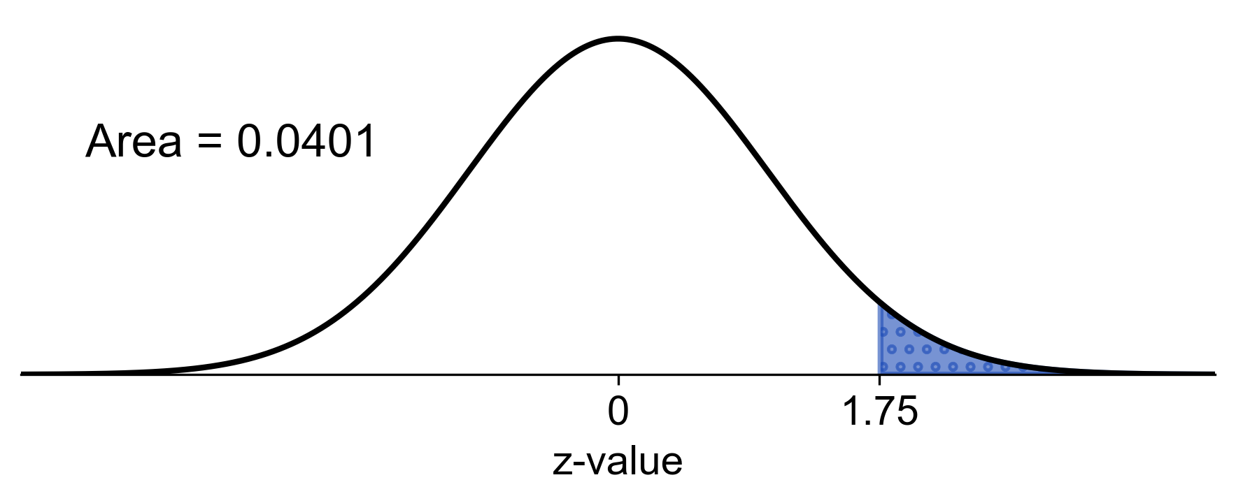
Fig. 5.74 Probability of a blood sugar reading greater than 120 mg/dL#
b) For the sample of 36 individuals, we calculate the z-scores for the mean blood sugar readings of 96 and 102 mg/dL and find the cumulative probability:
Using the standard normal distribution, we find the probability associated with \(-1.5 \leq Z \leq 1.5\).
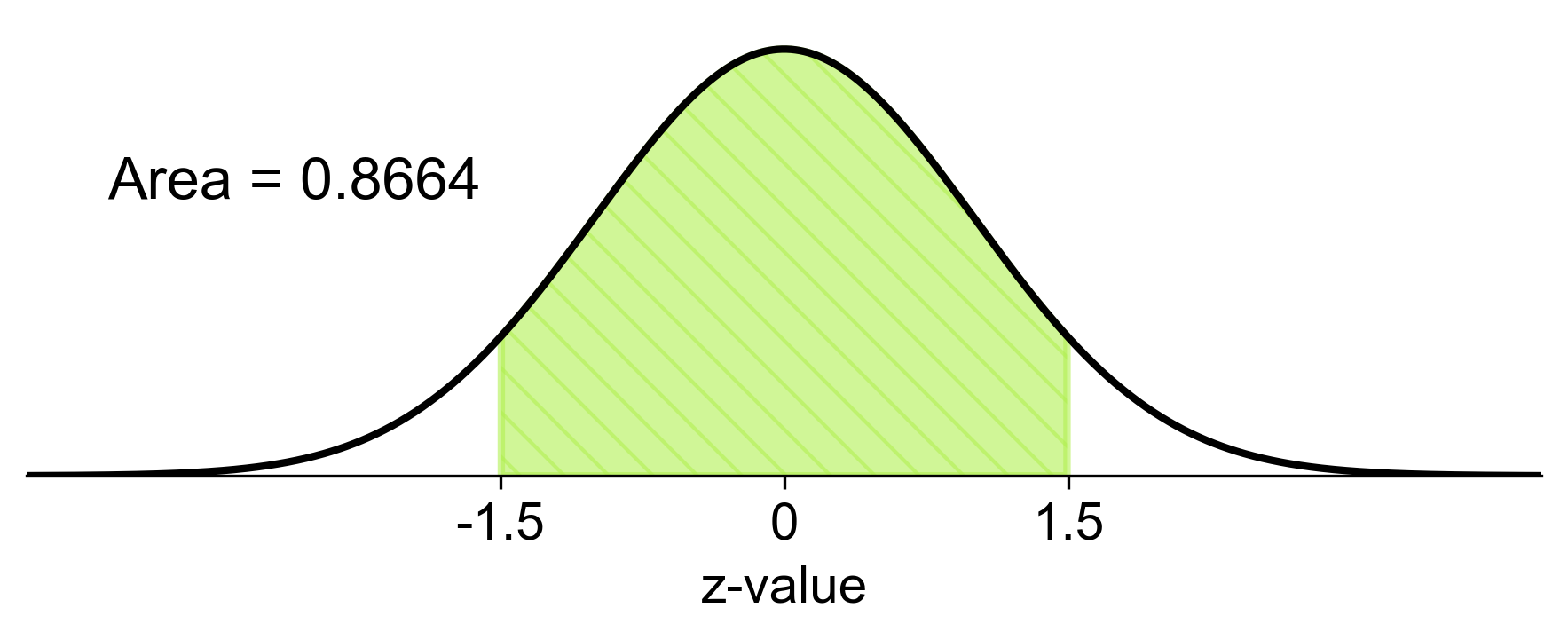
Fig. 5.75 Probability of average blood sugar reading between 96 and 102 mg/dL for a sample of 36 individuals#
Example 5.41
Assume the weights of women aged 16-30 are normally distributed with a mean (\(\mu\)) of 120 lbs and a standard deviation (\(\sigma\)) of 38 lbs. If a sample of \(n = 20\) women is selected at random from this population, determine the probability that the sample mean weight (\(\bar{X}\)) is:
a) Between 110 and 130 lbs.
b) Less than 115 lbs.
c) More than 120 lbs.
Solution:
a) To find the probability that the sample mean weight is between 110 and 130 lbs, we calculate the z-scores for both values and find the cumulative probability:
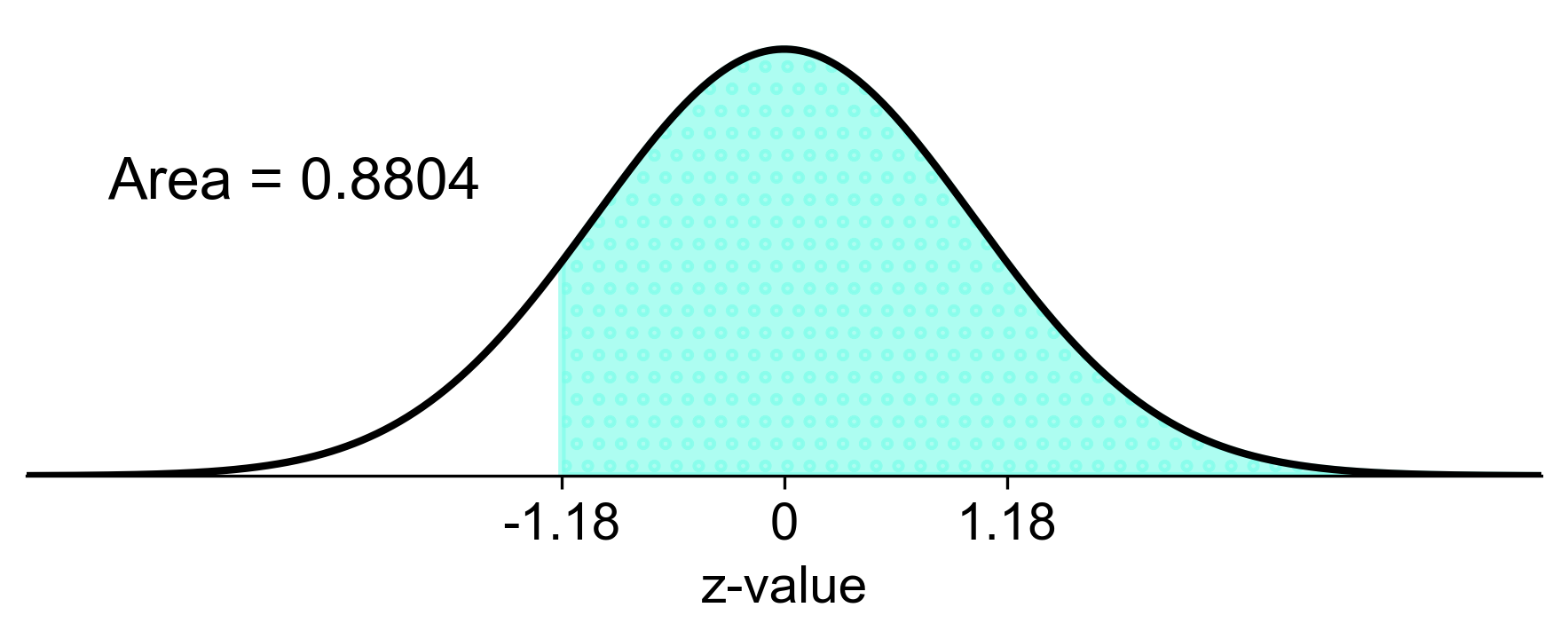
Fig. 5.76 Probability of sample mean weight between 110 and 130 lbs#
b) To find the probability that the sample mean weight is less than 115 lbs, we calculate the z-score for 115 lbs and use the standard normal distribution:
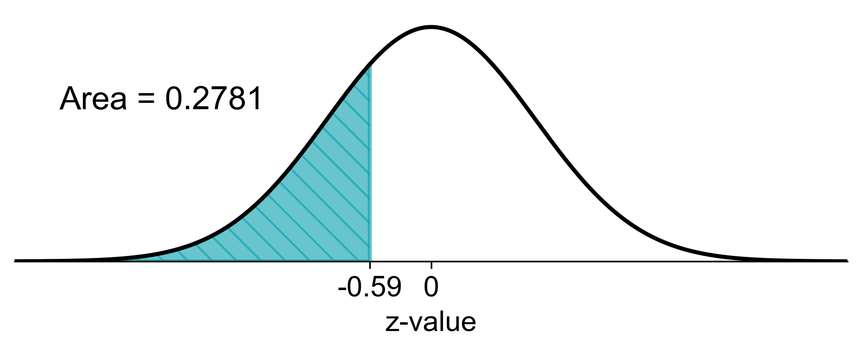
Fig. 5.77 Probability of sample mean weight less than 115 lbs#
c) To find the probability that the sample mean weight is more than 120 lbs, we note that since 120 lbs is the population mean, the z-score is 0:
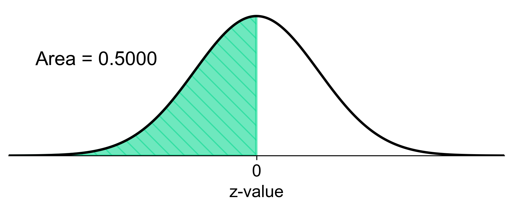
Fig. 5.78 Probability of sample mean weight more than 120 lbs#
This means:
a) There is a 76.08% chance that the average weight of a sample of 20 women will be between 110 and 130 lbs. b) There is a 27.81% chance that the average weight of a sample of 20 women will be less than 115 lbs. c) There is a 50% chance that the average weight of a sample of 20 women will be more than 120 lbs.
Example 5.42
A paleontologist has sampled the shell length of Devonian-age Paracyclas clams. It is believed that these shell lengths are normally distributed with a mean (\(\mu\)) of 45 mm and a standard deviation (\(\sigma\)) of 7.5 mm. In a random sample of \(n = 16\) shells, we want to determine the probability that the sample mean (\(\overline{X}\)) is:
a) Between 41 mm and 49 mm.
b) Less than or equal to 50 mm.
c) Greater than or equal to 45 mm.
d) Between 44.5 mm and 45.5 mm.
Solution:
a) The probability that the sample mean is between 41 mm and 49 mm is calculated using the z-score formula:
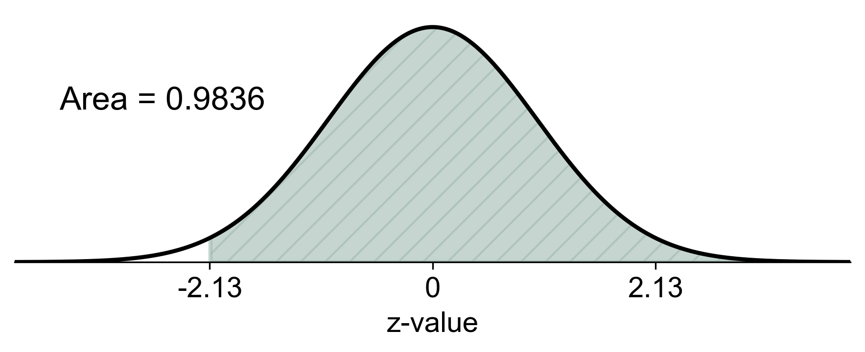
Fig. 5.79 Probability of sample mean shell length between 41 mm and 49 mm#
b) The probability that the sample mean is less than or equal to 50 mm is:
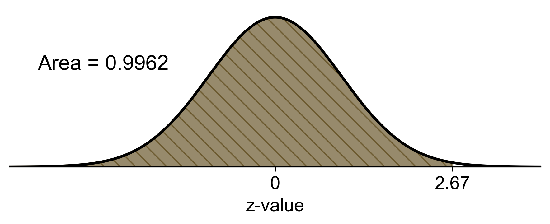
Fig. 5.80 Probability of sample mean shell length less than or equal to 50 mm#
c) The probability that the sample mean is greater than or equal to 45 mm (the population mean) is:
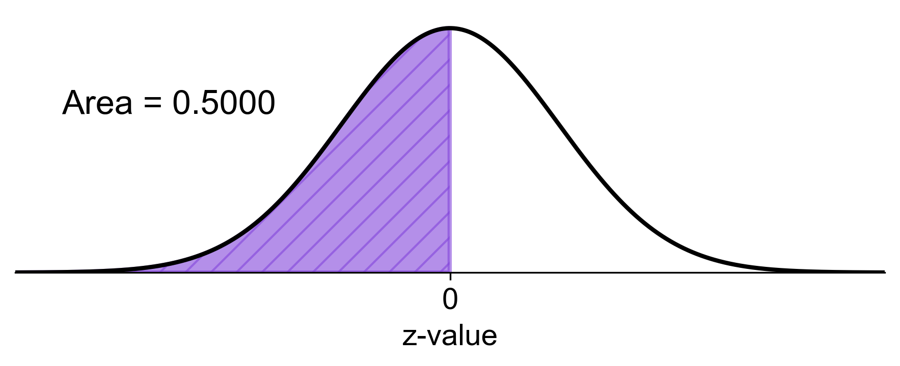
Fig. 5.81 Probability of sample mean shell length greater than or equal to 45 mm#
d) The probability that the sample mean is between 44.5 mm and 45.5 mm is:
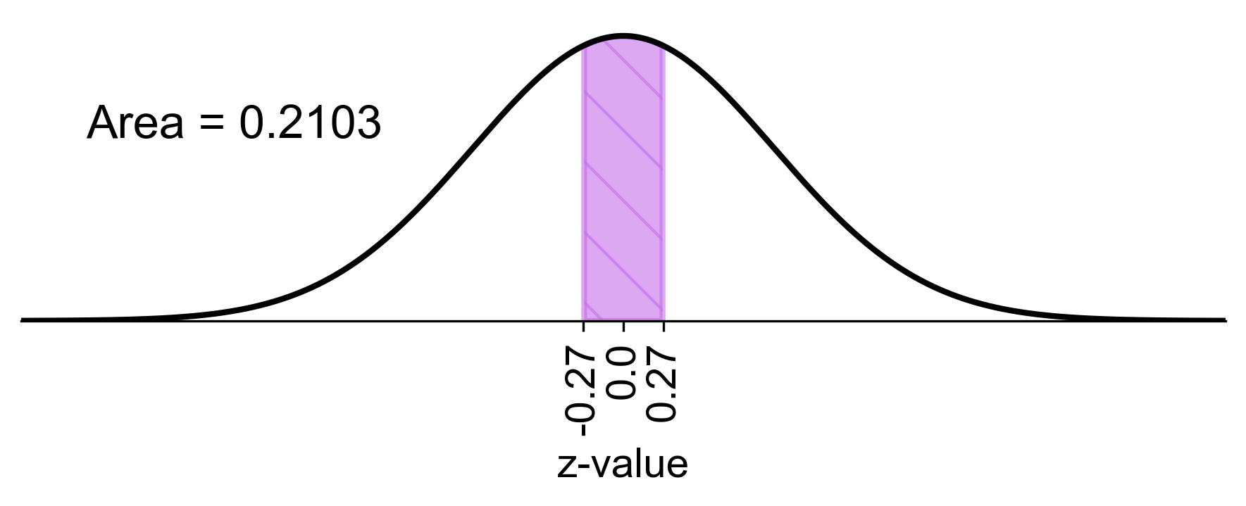
Fig. 5.82 Probability of sample mean shell length between 44.5 mm and 45.5 mm#
