7.5. P-Value#
Definition - P-Value
The P-value in a hypothesis test is a measure of the probability of obtaining sample data that is equal to or more extreme than the observed data, assuming that the null hypothesis is true. It provides evidence against the null hypothesis, with smaller P-values indicating stronger evidence. The notation \(P\) is commonly used to represent the P-value in statistical analyses.
7.5.1. Decision Criterion for a Hypothesis Test Using the P-Value#
In hypothesis testing, if the calculated P-value is less than or equal to the predetermined significance level (often denoted by \(\alpha\)), we reject the null hypothesis (\(H_{0}\)). Conversely, if the P-value is greater than \(\alpha\), we do not have enough evidence to reject the null hypothesis, and it remains valid for the given data.
In summary:
Reject \(H_{0}\) when \(P \leq \alpha\)
Do not reject \(H_{0}\) when \(P > \alpha\)
This decision criterion helps determine whether the observed data provides sufficient evidence to conclude that the null hypothesis is unlikely to be true.
7.5.2. P-Value as the Observed Significance Level#
The P-value of a hypothesis test represents the exact significance level at which the null hypothesis can be rejected. In other words, it is the smallest significance level for which the observed sample data leads to the rejection of \(H_{0}\). This interpretation allows researchers to understand the strength of the evidence against the null hypothesis.
7.5.3. Determining a P-Value#
To calculate the P-value of a hypothesis test, we assume that the null hypothesis is true and then assess the probability of observing a test statistic value that is as extreme as, or even more extreme than, the one we actually observed. By “extreme,” we refer to values that are significantly different from what we would expect if the null hypothesis were true.
The steps to determine a P-value typically involve:
Formulating the Null and Alternative Hypotheses: Define \(H_{0}\) and \(H_{a}\).
Calculating the Test Statistic: Based on the sample data, compute the value of the test statistic (e.g., z-score, t-score).
Finding the P-Value: Using the test statistic and the corresponding distribution (normal, t-distribution, etc.), find the probability of observing a value as extreme as, or more extreme than, the test statistic.
This process quantifies the strength of the evidence against the null hypothesis, guiding the decision on whether to reject \(H_{0}\).
7.5.4. Using the CDF in Hypothesis Testing#
From Section 5.1, we are familiar with the Cumulative Distribution Function (CDF). For a standard normal distribution (mean \(\mu = 0\) and standard deviation \(\sigma = 1\)), the CDF is denoted by \(F(z)\). It is often used to find p-values in hypothesis testing.
In hypothesis testing, the CDF is used to determine the p-value for a given test statistic \(z\):
Find the CDF value for the test statistic: \(F(z)\).
Calculate the p-value:
For a left-tailed test:
(7.3)#\[\begin{equation} \text{p-value} = F(z) = P(Z \leq z_{ts}), \end{equation}\]where \(z_{ts}\) represents the test statistic.
Fig. 7.8 illustrates how to find the p-value for a left-tailed test in statistics:
Shaded Area: The area to the left of the vertical dashed line (labeled as \(-z_{ts}\)) is shaded. This shaded region represents the p-value.
Equation: The equation \(\text{p-value} = F(z) = P(Z \leq z_{ts})\) indicates that the p-value is the cumulative probability from negative infinity up to the test statistic’s z-score (\(z_{ts}\)).
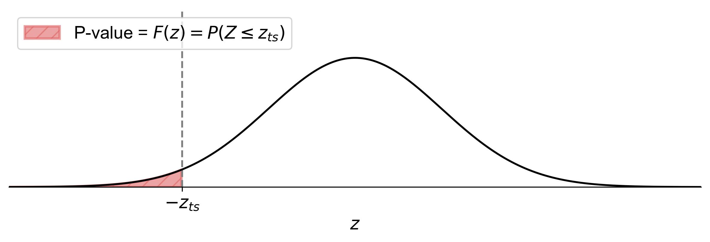
Fig. 7.8 Finding the p-value for a left-tailed test using the standard normal distribution curve.#
For a right-tailed test:
(7.4)#\[\begin{equation} \text{p-value} = 1 - F(z) = 1 - P(Z \leq z_{ts}), \end{equation}\]where \(z_{ts}\) represents the test statistic.
Fig. 7.9 illustrates how to find the p-value for a right-tailed test in statistics:
Shaded Area: The area to the right of the vertical dashed line (labeled as \(z_{ts}\)) is shaded. This shaded region represents the p-value.
Equation: The equation \(\text{p-value} = 1 - F(z) = 1 - P(Z \leq z_{ts})\) indicates that the p-value is the cumulative probability from the test statistic’s z-score (\(z_{ts}\)) to positive infinity.
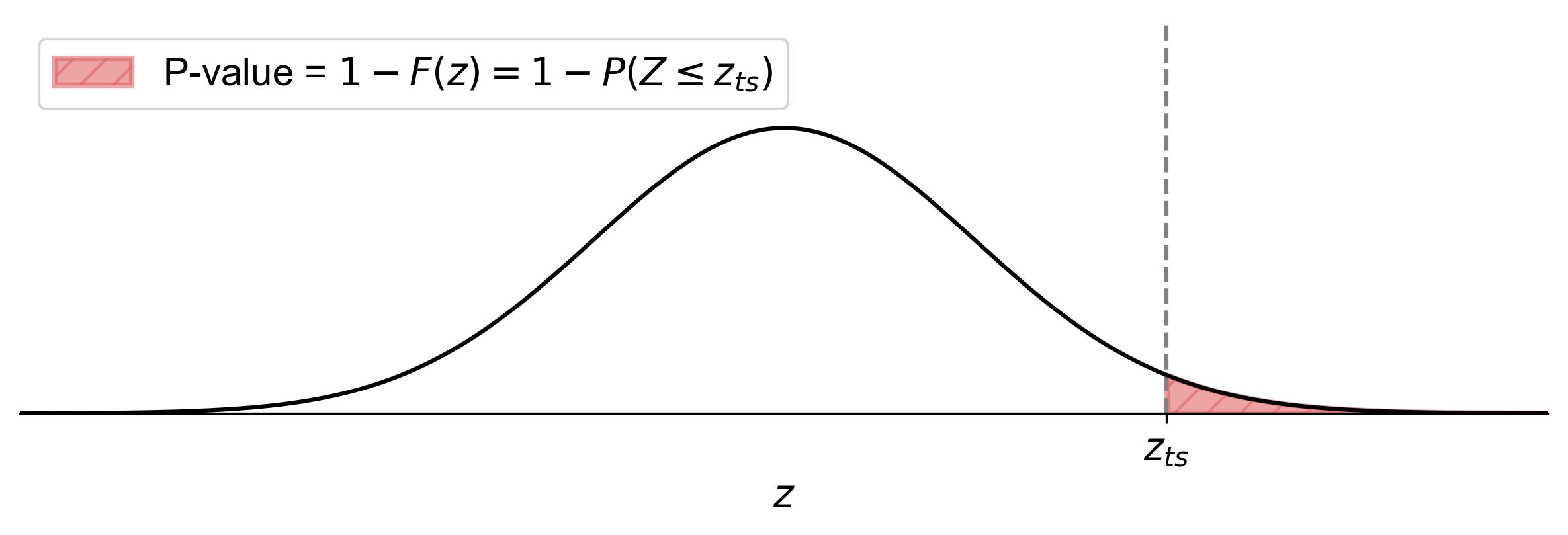
Fig. 7.9 Finding the p-value for a right-tailed test using the standard normal distribution curve.#
For a two-tailed test:
(7.5)#\[\begin{equation} \text{p-value} = 2 \times (1 - F(|z|)) = 2(1 - P(Z \leq |z_{ts}|)), \end{equation}\]where \(z_{ts}\) represents the test statistic.
Fig. 7.10 illustrates how to find the p-value for a two-tailed test in statistics:
Shaded Area: The areas to the left of \(-z_{ts}\) and to the right of \(z_{ts}\) are shaded. These shaded regions represent the p-value.
Equation: The equation \(\text{p-value} = 2 \times (1 - F(|z|)) = 2(1 - P(Z \leq |z_{ts}|))\) indicates that the p-value is twice the cumulative probability from the absolute value of the test statistic’s z-score (\(|z_{ts}|\)) to positive infinity.
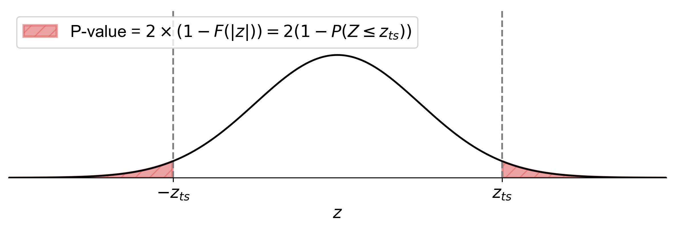
Fig. 7.10 Finding the p-value for a two-tailed test using the standard normal distribution curve.#
7.5.5. Finding the P-Value Using a Z-Distribution Table#
To find the p-value using a z-distribution table, follow these steps:
Locate the Z-Score: Find the corresponding z-score in the z-distribution table.
Determine the Cumulative Probability: The table provides the cumulative probability up to the z-score.
Calculate the P-Value:
For a left-tailed test, the p-value is the cumulative probability from the table.
For a right-tailed test, subtract the cumulative probability from 1.
For a two-tailed test, multiply the smaller tail probability by 2.
This method helps quantify the evidence against the null hypothesis by using the standard normal distribution.
Example 7.21
Given a test statistic of \(z = 2.05\) for a one-tailed test and a significance level \(\alpha = 0.05\), find the p-value and compare it against the significance level to determine whether to reject the null hypothesis (\(H_0\)).
Solution:
Calculate the p-value:
The p-value represents the probability of obtaining a test statistic at least as extreme as the observed value, assuming the null hypothesis is true.
For a z-test, the p-value for a test statistic \(z\) is \(P(Z \geq 2.05)\).
Using the cumulative distribution function (CDF) for the standard normal distribution, the p-value is:
\[\begin{equation*} \text{p-value} = 1 - F(2.05) = 1 - 0.9798 = 0.0202 \end{equation*}\]
Compare the p-value with \(\alpha\):
\(\text{p-value} = 0.0202\)
\(\alpha = 0.05\)
Since \(\text{p-value} < \alpha\), we reject \(H_0\).
Fig. 7.11 illustrates the one-tailed hypothesis test for this example:
The bell curve represents the standard normal distribution under the null hypothesis.
The vertical red line at \(z = 1.645\) represents the critical value for a one-tailed test at \(\alpha = 0.05\).
The shaded area to the right of the critical value represents the rejection region, which has an area of 0.05 (5%).
The vertical blue line at \(z = 2.05\) represents our calculated test statistic.
The darker shaded area to the right of the test statistic represents the p-value, which is 0.0202 (2.02%).
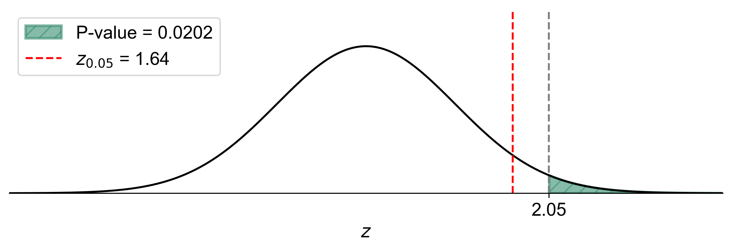
Fig. 7.11 Visualization of One-Tailed Hypothesis Test with p-value#
This visual representation clearly shows that our test statistic (\(z = 2.05\)) falls within the rejection region, and the p-value (the area to the right of the blue line) is smaller than the significance level \(\alpha = 0.05\) (the total shaded area). This supports our conclusion to reject the null hypothesis.
The figure helps us visualize why we reject \(H_0\): the probability of observing a test statistic this extreme or more extreme (the p-value) is less than our predetermined threshold for rejecting \(H_0\) (the significance level \(\alpha\)). This graphical representation reinforces our analytical conclusion and provides an intuitive understanding of the relationship between the test statistic, p-value, and significance level in hypothesis testing.
Example 7.22
Given a test statistic of \(z = 1.65\) for a one-tailed test and a significance level \(\alpha = 0.10\), find the p-value and compare it against the significance level to determine whether to reject the null hypothesis (\(H_0\)).
Solution:
Calculate the p-value:
The p-value represents the probability of obtaining a test statistic at least as extreme as the observed value, assuming the null hypothesis is true.
For a z-test, the p-value for a test statistic \(z\) is \(P(Z \geq 1.65)\).
Using the cumulative distribution function (CDF) for the standard normal distribution, the p-value is:
\[\begin{equation*} \text{p-value} = 1 - F(1.65) = 1 - 0.9505 = 0.0495 \end{equation*}\]
Compare the p-value with \(\alpha\):
\(\text{p-value} = 0.0495\)
\(\alpha = 0.10\)
Since \(\text{p-value} < \alpha\), we reject \(H_0\).
Fig. 7.12 illustrates the one-tailed hypothesis test for this example:
The bell curve represents the standard normal distribution under the null hypothesis.
The vertical red line at \(z = 1.28\) represents the critical value for a one-tailed test at \(\alpha = 0.10\).
The shaded area to the right of the critical value represents the rejection region, which has an area of 0.10 (10%).
The vertical blue line at \(z = 1.65\) represents our calculated test statistic.
The darker shaded area to the right of the test statistic represents the p-value, which is 0.0495 (4.95%).
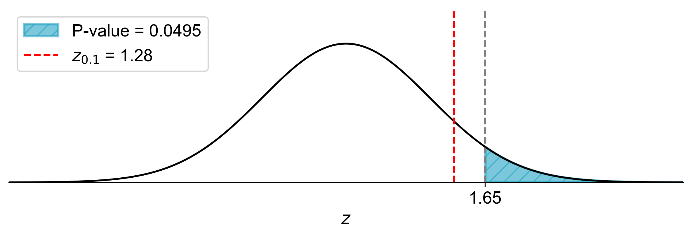
Fig. 7.12 Visualization of One-Tailed Hypothesis Test with p-value#
This visual representation clearly shows that our test statistic (\(z = 1.65\)) falls within the rejection region, and the p-value (the area to the right of the blue line) is smaller than the significance level \(\alpha = 0.10\) (the total shaded area). This supports our conclusion to reject the null hypothesis.
The figure helps us visualize why we reject \(H_0\): the probability of observing a test statistic this extreme or more extreme (the p-value) is less than our predetermined threshold for rejecting \(H_0\) (the significance level \(\alpha\)). In this case, we can see that the test statistic is well into the rejection region, and the p-value is considerably smaller than \(\alpha\), providing strong evidence against the null hypothesis.
This graphical representation reinforces our analytical conclusion and provides an intuitive understanding of the relationship between the test statistic, p-value, and significance level in hypothesis testing. It also illustrates how a larger significance level (\(\alpha = 0.10\) in this case) results in a wider rejection region compared to more commonly used levels like 0.05 or 0.01.
Example 7.23
Given a test statistic of \(z = 2.50\) for a two-tailed test and a significance level \(\alpha = 0.05\), find the p-value and compare it against the significance level to determine whether to reject the null hypothesis (\(H_0\)).
Solution:
Calculate the p-value:
The p-value represents the probability of obtaining a test statistic at least as extreme as the observed value, assuming the null hypothesis is true.
For a two-tailed z-test, the p-value for a test statistic \(z\) is \(2 \times P(Z \geq |2.50|)\).
Using the cumulative distribution function (CDF) for the standard normal distribution, the p-value is:
\[\begin{equation*} \text{p-value} = 2 \times (1 - F(2.50)) = 2 \times (1 - 0.9938) = 2 \times 0.0062 = 0.0124 \end{equation*}\]
Compare the p-value with \(\alpha\):
\(\text{p-value} = 0.0124\)
\(\alpha = 0.05\)
Since \(\text{p-value} < \alpha\), we reject \(H_0\).
Fig. 7.13 illustrates the two-tailed hypothesis test for this example:
The bell curve represents the standard normal distribution under the null hypothesis.
The vertical red lines at \(z = \pm 1.96\) represent the critical values for a two-tailed test at \(\alpha = 0.05\).
The shaded areas to the left of \(-1.96\) and to the right of \(1.96\) represent the rejection regions, which together have an area of 0.05 (5%).
The vertical blue lines at \(z = \pm 2.50\) represent our calculated test statistic and its negative counterpart.
The darker shaded areas to the left of \(-2.50\) and to the right of \(2.50\) represent the p-value, which is 0.0124 (1.24%).
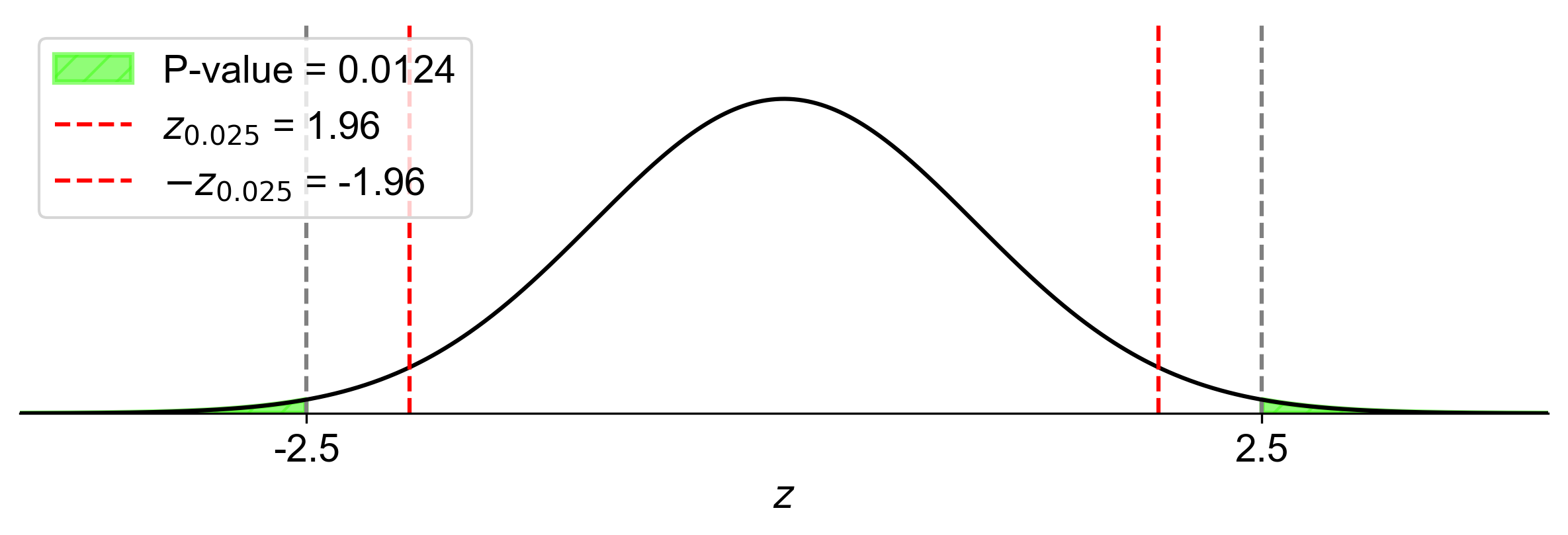
Fig. 7.13 Visualization of Two-Tailed Hypothesis Test with p-value#
This visual representation clearly shows that our test statistic (\(z = 2.50\)) falls within the rejection region, and the p-value (the total area of the darker shaded regions) is smaller than the significance level \(\alpha = 0.05\) (the total area of all shaded regions). This supports our conclusion to reject the null hypothesis.
The figure helps us visualize why we reject \(H_0\) in a two-tailed test:
The test statistic is more extreme than the critical values in both directions.
The probability of observing a test statistic this extreme or more extreme in either direction (the p-value) is less than our predetermined threshold for rejecting \(H_0\) (the significance level \(\alpha\)).
Example 7.24
Given a test statistic of \(z = -2.30\) for a two-tailed test and a significance level \(\alpha = 0.01\), find the p-value and compare it against the significance level to determine whether to reject the null hypothesis (\(H_0\)).
Solution:
Calculate the p-value:
The p-value represents the probability of obtaining a test statistic at least as extreme as the observed value, assuming the null hypothesis is true.
For a two-tailed z-test, the p-value for a test statistic \(z\) is \(2 \times P(Z \geq |2.30|)\).
Using the cumulative distribution function (CDF) for the standard normal distribution, the p-value is:
\[\begin{equation*} \text{p-value} = 2 \times (1 - F(2.30)) = 2 \times (1 - 0.9893) = 2 \times 0.0107 = 0.0214 \end{equation*}\]
Compare the p-value with \(\alpha\):
\(\text{p-value} = 0.0214\)
\(\alpha = 0.01\)
Since \(\text{p-value} > \alpha\), we do not reject \(H_0\).
Fig. 7.14 illustrates the two-tailed hypothesis test for this example:
The bell curve represents the standard normal distribution under the null hypothesis.
The vertical red lines at \(z = \pm 2.576\) represent the critical values for a two-tailed test at \(\alpha = 0.01\).
The shaded areas to the left of \(-2.576\) and to the right of \(2.576\) represent the rejection regions, which together have an area of 0.01 (1%).
The vertical blue lines at \(z = \pm 2.30\) represent our calculated test statistic and its positive counterpart.
The darker shaded areas to the left of \(-2.30\) and to the right of \(2.30\) represent the p-value, which is 0.0214 (2.14%).
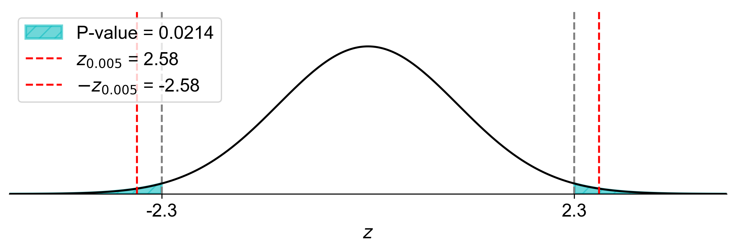
Fig. 7.14 Visualization of Two-Tailed Hypothesis Test with p-value#
This visual representation clearly shows that our test statistic (\(z = -2.30\)) falls outside the rejection region, and the p-value (the total area of the darker shaded regions) is larger than the significance level \(\alpha = 0.01\) (the total area of all shaded regions). This supports our conclusion to not reject the null hypothesis.
The figure helps us visualize why we do not reject \(H_0\) in this two-tailed test:
The test statistic, while extreme, is not more extreme than the critical values in both directions.
The probability of observing a test statistic this extreme or more extreme in either direction (the p-value) is greater than our predetermined threshold for rejecting \(H_0\) (the significance level \(\alpha\)).
In this case, we can see that the test statistic is close to, but not within, the rejection region, and the p-value is larger than \(\alpha\), indicating that we don’t have sufficient evidence to reject the null hypothesis at this significance level.
This graphical representation reinforces our analytical conclusion and provides an intuitive understanding of the relationship between the test statistic, p-value, and significance level in two-tailed hypothesis testing. It illustrates how a smaller significance level (\(\alpha = 0.01\) in this case) results in a narrower rejection region compared to more commonly used levels like 0.05, making it harder to reject the null hypothesis.
Example 7.25
Given a test statistic of \(z = 1.75\) for a one-tailed test and a significance level \(\alpha = 0.10\), find the p-value and compare it against the significance level to determine whether to reject the null hypothesis (\(H_0\)).
Solution:
Calculate the p-value:
The p-value represents the probability of obtaining a test statistic at least as extreme as the observed value, assuming the null hypothesis is true.
For a one-tailed z-test, the p-value for a test statistic \(z\) is \(P(Z \geq 1.75)\).
Using the cumulative distribution function (CDF) for the standard normal distribution, the p-value is:
\[\begin{equation*} \text{p-value} = 1 - F(1.75) = 1 - 0.9599 = 0.0401 \end{equation*}\]
Compare the p-value with \(\alpha\):
\(\text{p-value} = 0.0401\)
\(\alpha = 0.10\)
Since \(\text{p-value} < \alpha\), we reject \(H_0\).
Fig. 7.15 illustrates the one-tailed hypothesis test for this example:
The bell curve represents the standard normal distribution under the null hypothesis.
The vertical red line at \(z = 1.28\) represents the critical value for a one-tailed test at \(\alpha = 0.10\).
The shaded area to the right of the critical value represents the rejection region, which has an area of 0.10 (10%).
The vertical blue line at \(z = 1.75\) represents our calculated test statistic.
The darker shaded area to the right of the test statistic represents the p-value, which is 0.0401 (4.01%).
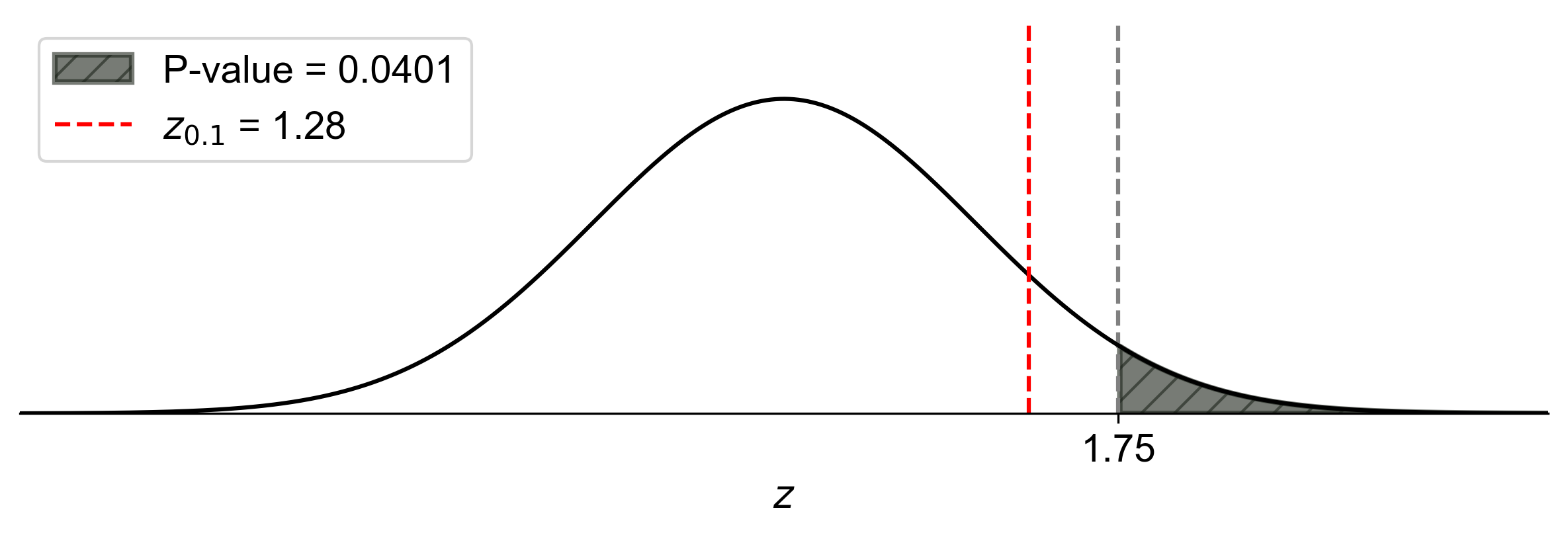
Fig. 7.15 Visualization of One-Tailed Hypothesis Test with p-value#
This visual representation clearly shows that our test statistic (\(z = 1.75\)) falls within the rejection region, and the p-value (the area to the right of the blue line) is smaller than the significance level \(\alpha = 0.10\) (the total shaded area). This supports our conclusion to reject the null hypothesis.
The figure helps us visualize why we reject \(H_0\):
The test statistic is more extreme than the critical value.
The probability of observing a test statistic this extreme or more extreme (the p-value) is less than our predetermined threshold for rejecting \(H_0\) (the significance level \(\alpha\)).
In this case, we can see that the test statistic is well into the rejection region, and the p-value is considerably smaller than \(\alpha\), providing strong evidence against the null hypothesis.
This graphical representation reinforces our analytical conclusion and provides an intuitive understanding of the relationship between the test statistic, p-value, and significance level in one-tailed hypothesis testing. It illustrates how a larger significance level (\(\alpha = 0.10\) in this case) results in a wider rejection region compared to more commonly used levels like 0.05 or 0.01, making it easier to reject the null hypothesis.
7.5.6. Using the CDF in Hypothesis Testing with T-Score#
For a t-distribution, the CDF is denoted by \(F(t)\). It is often used to find p-values in hypothesis testing.
In hypothesis testing, the CDF is used to determine the p-value for a given test statistic \(t\):
Find the CDF value for the test statistic: \(F(t)\).
Calculate the p-value:
For a left-tailed test:
(7.6)#\[\begin{equation} \text{p-value} = F(t) = P(T \leq t_{ts,df}), \end{equation}\]where \(t_{ts,df}\) represents the test statistic.
Fig. 7.16 illustrates how to find the p-value for a left-tailed test in statistics:
Shaded Area: The area to the left of the vertical dashed line (labeled as \(-t_{ts,df}\)) is shaded. This shaded region represents the p-value.
Equation: The equation \(\text{p-value} = F(t) = P(T \leq t_{ts,df})\) indicates that the p-value is the cumulative probability from negative infinity up to the test statistic’s t-score (\(t_{ts,df}\)).
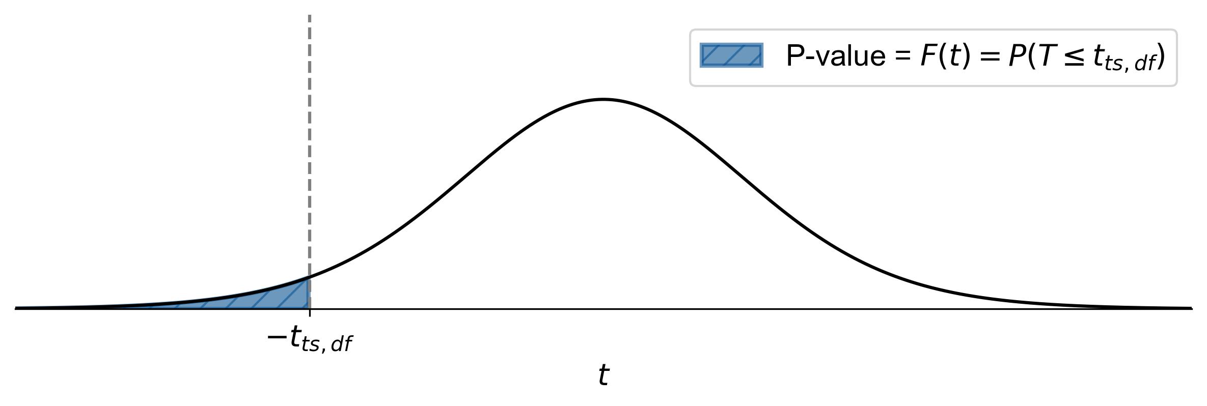
Fig. 7.16 Finding the p-value for a left-tailed test using the t-distribution curve.#
For a right-tailed test:
(7.7)#\[\begin{equation} \text{p-value} = 1 - F(t) = 1 - P(T \leq t_{ts,df}), \end{equation}\]where \(t_{ts,df}\) represents the test statistic.
Fig. 7.17 illustrates how to find the p-value for a right-tailed test in statistics:
Shaded Area: The area to the right of the vertical dashed line (labeled as \(t_{ts,df}\)) is shaded. This shaded region represents the p-value.
Equation: The equation \(\text{p-value} = 1 - F(t) = 1 - P(T \leq t_{ts,df})\) indicates that the p-value is the cumulative probability from the test statistic’s t-score (\(t_{ts,df}\)) to positive infinity.
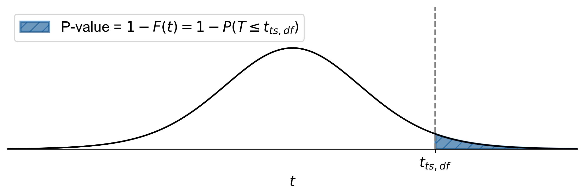
Fig. 7.17 Finding the p-value for a right-tailed test using the t-distribution curve.#
For a two-tailed test:
(7.8)#\[\begin{equation} \text{p-value} = 2 \times (1 - F(|t|)) = 2(1 - P(T \leq |t_{ts,df}|)), \end{equation}\]where \(t_{ts,df}\) represents the test statistic.
Fig. 7.18 illustrates how to find the p-value for a two-tailed test in statistics:
Shaded Area: The areas to the left of \(-t_{ts,df}\) and to the right of \(t_{ts,df}\) are shaded. These shaded regions represent the p-value.
Equation: The equation \(\text{p-value} = 2 \times (1 - F(|t|)) = 2(1 - P(T \leq |t_{ts,df}|))\) indicates that the p-value is twice the cumulative probability from the absolute value of the test statistic’s t-score (\(|t_{ts,df}|\)) to positive infinity.
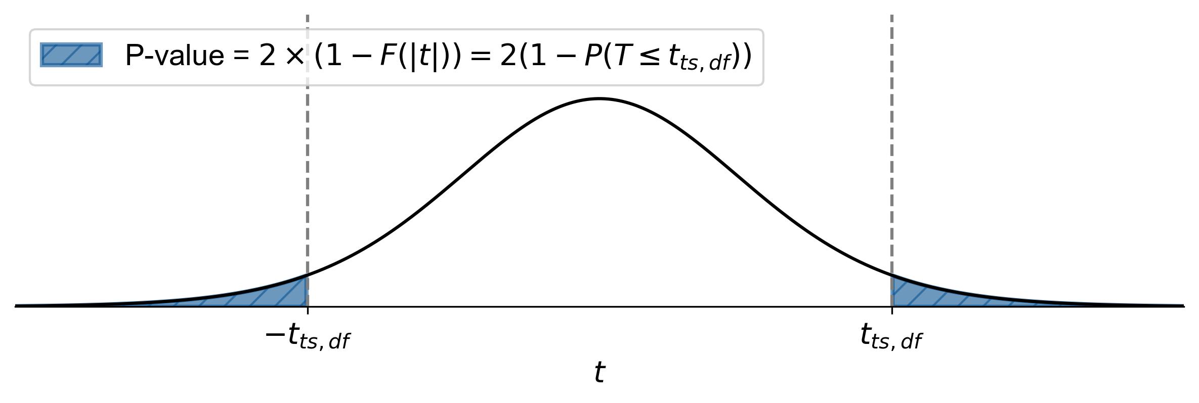
Fig. 7.18 Finding the p-value for a two-tailed test using the t-distribution curve.#
7.5.7. Estimating p-value Using a t-Distribution Table#
To estimate the p-value using a t-distribution table, follow these steps:
Determine Degrees of Freedom (df): Calculate the degrees of freedom, which is \(n - 1\) for a one-sample t-test (we will discuss it in Section 7.8).
Locate the t-Statistic in the Table: Find the row corresponding to your degrees of freedom and locate the range in which your t-statistic falls.
Estimate the p-value: Identify the significance level (\(\alpha\)) columns that bracket your t-statistic. The p-value is between these two significance levels.
Example 7.26
Suppose we have a one-tailed test, sample size of 15 and a t-Statistic of \(3.572\).
Fig. 7.19 illustrates how to find the p-value:
Degrees of Freedom:
Locate the t-Statistic in the Table: For \(df = 14\), the t-statistic of 3.572 falls between the critical values for \(\alpha = 0.005\) (2.977) and \(\alpha = 0.001\) (3.787).
Estimate the p-value: The p-value is between 0.005 and 0.001.
This means there is a very low probability (less than 0.5%) that the observed difference is due to random chance, leading to the rejection of the null hypothesis at common significance levels.

Fig. 7.19 Finding the p-value for a one-tailed test, sample size of 15 and a t-Statistic of \(3.872\).#
Relationship Between Test Statistic and P-Value
Definitions:
The test statistic (e.g., z-value, t-value) is a standardized measure indicating the degree to which the sample data deviates from the null hypothesis.
The p-value quantifies the probability of observing a test statistic as extreme as, or more extreme than, the one calculated, assuming the null hypothesis is true.
Key Relationship:
Larger Test Statistics:
Indicate greater deviation from the null hypothesis.
Correspond to smaller p-values, suggesting stronger evidence against the null hypothesis.
Example: A z-value of 2.5 yields a p-value of approximately 0.006, compared to a z-value of 1.5, which results in a p-value around 0.133. Similarly, a t-value of 3.0 produces a smaller p-value than a t-value of 1.0.
Smaller Test Statistics:
Indicate that the sample data aligns more closely with the null hypothesis.
Correspond to larger p-values, indicating weaker evidence against the null hypothesis.
Example: A z-value of 0.5 corresponds to a p-value of approximately 0.308, while a z-value of 1.0 corresponds to about 0.158. For t-values, smaller values yield similarly larger p-values.
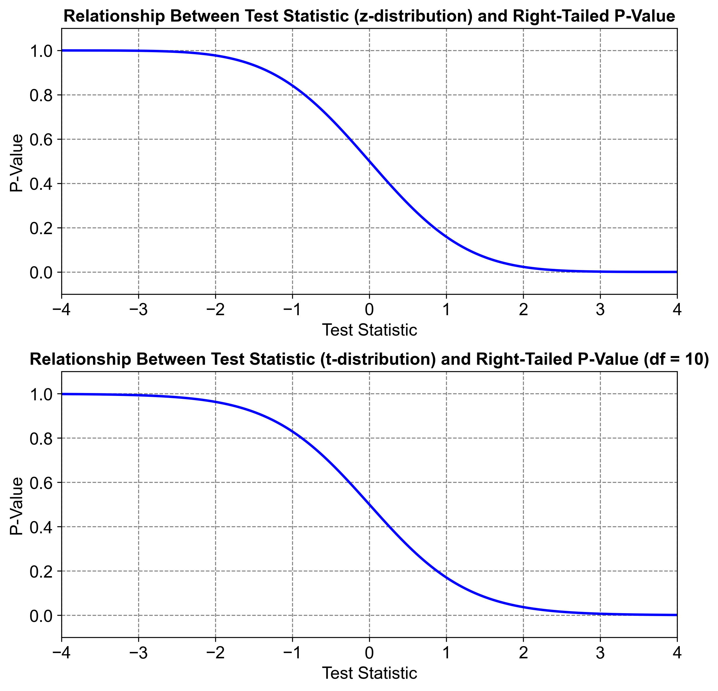
Fig. 7.20 Relationship between p-value and test statistic.#
Fig. 7.20 demonstrates the inverse relationship between test statistics and p-values, where larger test statistics correspond to smaller p-values, indicating stronger evidence against the null hypothesis. The relationship between test statistics and p-values is depicted in two graphs. The top graph shows a z-distribution, while the bottom graph illustrates a t-distribution with 10 degrees of freedom. Both graphs demonstrate an inverse relationship: as the test statistic increases, the p-value decreases. This inverse relationship is crucial in hypothesis testing, where larger test statistics suggest stronger evidence against the null hypothesis, resulting in smaller p-values, and vice versa. This understanding helps determine whether to reject or fail to reject the null hypothesis based on the significance level.
