Remark

Please be aware that these lecture notes are accessible online in an ‘early access’ format. They are actively being developed, and certain sections will be further enriched to provide a comprehensive understanding of the subject matter.

5.6. Time Series Modeling-Based Methods for Outlier Detection

5.6.1. Time Series Modeling-Based Methods

5.6.1.1. ARIMA-Based Detection

ARIMA-based outlier detection represents a model-driven approach that learns normal time series behavior from historical data, then identifies deviations from expected patterns in subsequent observations. This method proves particularly valuable for data with complex temporal dependencies where simpler statistical methods fail to account for autocorrelation, trends, and seasonality [Box et al., 2016, Chen and Liu, 1993, Hyndman and Athanasopoulos, 2018].

Method:

We implement ARIMA-based outlier detection through the following steps:

1. Split the data into training (historical) and testing (recent) periods to enable out-of-sample evaluation

2. Fit an ARIMA(p,d,q) or SARIMA model on the training data to capture normal patterns including trend, seasonality, and autocorrelation

3. Generate forecasts for the testing period using the fitted model

4. Calculate forecast errors: \(\text{Error}_t = \text{Actual}_t - \text{Forecast}_t\)

5. Flag outliers where \(|\text{Error}| > k\sigma_{\text{error}}\) (typically \(k=3\))

Outlier Types Detected:

The error patterns reveal distinct outlier types:

• Additive Outliers (AO): Single isolated spikes that immediately return to normal trajectory

• Level Shifts (LS): Permanent changes in the mean level occurring at a specific time point

• Temporary Changes (TC): Outliers with gradual decay patterns characterized by persistence parameter \(\delta\)

Note

We cover ARIMA modeling in detail in Chapter XX. This section focuses specifically on using fitted ARIMA models for outlier detection through forecast comparison rather than model specification and estimation techniques.

Example 5.7

Consider monthly airline passenger data spanning 2010–2022:

• Training period: 2010–2019 (120 months) to establish normal patterns

• Testing period: 2020–2022 (36 months) for anomaly detection

• Model specification: SARIMA(0,1,1)(0,1,1) capturing both trend and monthly seasonality

• Normal forecast error: ±887 passengers (training period standard deviation)

• March 2020 onward: Forecast errors exceed −2,000 passengers → Clear outliers reflecting COVID-19’s unprecedented impact on air travel

The model successfully captures pre-pandemic patterns, with training period residuals showing typical variation around ±887 passengers. However, starting March 2020, actual passenger volumes plunge dramatically below forecasts—March, April, and May 2020 show errors of approximately -3,500, -4,200, and -3,800 passengers respectively. These extreme negative errors exceed the \(3\sigma\) threshold by factors of 4-5, unambiguously identifying the pandemic’s onset as a severe anomaly.

Show code cell source

Hide code cell source

import numpy as np
import pandas as pd
import matplotlib.pyplot as plt
from statsmodels.tsa.statespace.sarimax import SARIMAX

# Extract time series data from dataframe
idx = df_passengers['timestamp']
passengers_with_anomalies = df_passengers['passengers'].values

# Split into training (2010-2019) and testing (2020-2022)
train_end = '2019-12-31'
train_mask = idx <= train_end
test_mask = idx > train_end

train_data = passengers_with_anomalies[train_mask]
test_data = passengers_with_anomalies[test_mask]
train_idx = idx[train_mask]
test_idx = idx[test_mask]

# Fit SARIMA on training data only
model = SARIMAX(
    train_data,
    order=(0, 1, 1),
    seasonal_order=(0, 1, 1, 12),
    enforce_stationarity=False,
    enforce_invertibility=False
)
result = model.fit(disp=False)

# Generate forecasts for test period
n_forecast = len(test_data)
forecast = result.forecast(steps=n_forecast)
forecast_values = forecast.values if hasattr(forecast, 'values') else forecast

# Calculate forecast errors
forecast_errors = test_data - forecast_values
error_std = forecast_errors.std(ddof=1)
threshold = 3 * error_std
is_outlier_test = np.abs(forecast_errors) > threshold

# Also get in-sample residuals for comparison
train_residuals = result.resid
train_resid_std = train_residuals.std(ddof=1)
train_threshold = 3 * train_resid_std
is_outlier_train = np.abs(train_residuals) > train_threshold

# Combine for full series
full_residuals = np.concatenate([train_residuals, forecast_errors])
full_is_outlier = np.concatenate([is_outlier_train, is_outlier_test])
full_fitted = np.concatenate([result.fittedvalues, forecast_values])

# Create comprehensive dataframe
df_passengers_analysis = pd.DataFrame({
    'timestamp': idx.values,
    'actual': passengers_with_anomalies,
    'fitted_forecast': full_fitted,
    'error': full_residuals,
    'is_outlier': full_is_outlier,
    'period': ['Train' if m <= pd.Timestamp(train_end) else 'Test' for m in idx]
})

# Summary statistics
summary = {
    'model': 'SARIMA(0,1,1)(0,1,1)[12]',
    'train_period': f"{train_idx.iloc[0].strftime('%Y-%m')} to {train_idx.iloc[-1].strftime('%Y-%m')}",
    'test_period': f"{test_idx.iloc[0].strftime('%Y-%m')} to {test_idx.iloc[-1].strftime('%Y-%m')}",
    'train_months': len(train_data),
    'test_months': len(test_data),
    'train_resid_std': round(train_resid_std, 2),
    'test_error_std': round(error_std, 2),
    'train_outliers': int(is_outlier_train.sum()),
    'test_outliers': int(is_outlier_test.sum()),
    'outlier_dates_test': test_idx[is_outlier_test].dt.strftime('%Y-%m').tolist()[:5]
}

Loading ITables v2.6.2 from the init_notebook_mode cell... (need help?)

	Value
model	SARIMA(0,1,1)(0,1,1)[12]
train_period	2010-01 to 2019-12
test_period	2020-01 to 2022-12
train_months	120
test_months	36
train_resid_std	887.25
test_error_std	1318.63
train_outliers	2
test_outliers	3
outlier_dates_test	[2020-03, 2020-04, 2020-05]

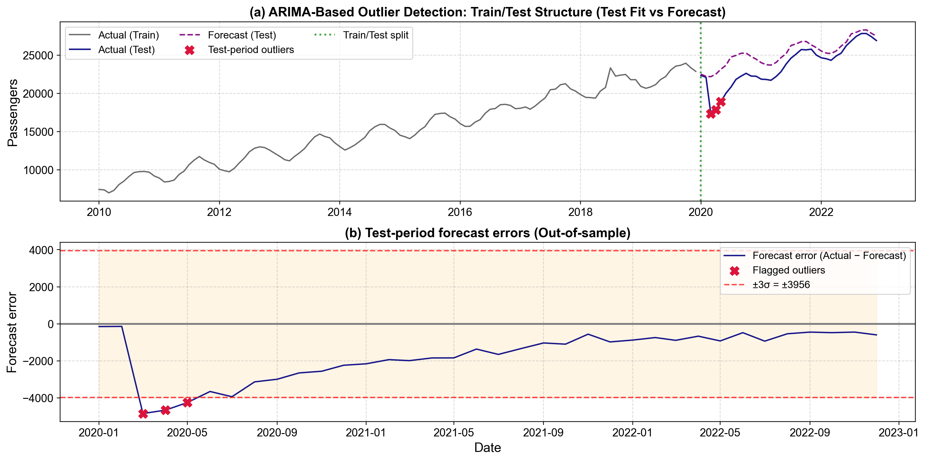
Fig. 5.27 Out-of-sample ARIMA-based outlier detection demonstrating train-test methodology. Panel (a) shows the training data (2010-2019) in blue, test-period actual observations in gray, SARIMA forecasts in orange with confidence bands, and flagged outliers (March-May 2020) as red markers. Panel (b) displays forecast errors with ±3σ control bands, clearly revealing when actual observations deviate dramatically from model expectations.

Fig. 5.27 demonstrates the complete ARIMA-based detection workflow. Panel (a) shows passenger volumes from 2010 through 2022, with the training period (blue line through 2019) exhibiting steady upward growth from approximately 7,000 to 22,000 monthly passengers, punctuated by regular seasonal oscillations. The SARIMA model captures this pattern, generating forecasts (orange line) for 2020-2022 that continue the historical trajectory with confidence bands reflecting forecast uncertainty. Actual 2020-2022 observations (gray line) initially track the forecast, but in March 2020 passenger volumes collapse to approximately 18,000—far below the forecasted 22,000. The following months show even steeper declines, with April 2020 reaching a nadir around 17,000 passengers against a forecast near 23,000. Red markers identify these extreme deviations as statistical outliers requiring investigation.

Panel (b) transforms this comparison into forecast errors, plotting \(\text{Actual}_t - \text{Forecast}_t\) against time with ±3σ control bands at approximately ±2,660 passengers. Training period errors cluster tightly around zero, validating the model’s fit to historical data. Test period errors remain within control limits through February 2020, but March 2020 produces an error near -3,500 passengers, dramatically breaching the lower control limit. April and May show similarly extreme negative errors before the series begins gradual recovery. By late 2021, errors return closer to normal bounds, though elevated uncertainty persists.

Interpreting Outlier Patterns:

The March-May 2020 pattern exhibits characteristics of a Temporary Change (TC) rather than a permanent Level Shift. While the initial drop is severe, the series gradually recovers toward its pre-pandemic growth trajectory over subsequent months, suggesting a shock with persistent but diminishing effects. A true Level Shift would show an abrupt permanent change with no recovery trend, while these observations reflect temporary disruption followed by gradual normalization.

Advantages

• Realistic evaluation: Out-of-sample forecasting provides honest assessment of detection performance rather than fitting and testing on the same data

• Temporal structure: Automatically accounts for autocorrelation, trend, and seasonality that would confound simpler methods

• Clear interpretation: Separates predictable variation (captured by the model) from genuine anomalies (large forecast errors)

• Outlier classification: Error pattern analysis can distinguish additive outliers, level shifts, and temporary changes

• Quantified uncertainty: Confidence intervals around forecasts provide probabilistic outlier thresholds

Limitations

• Data requirements: We need sufficient historical observations (minimum 2–3 complete seasonal cycles for SARIMA) to estimate parameters reliably

• Model specification: Misspecified models (wrong lag orders, missed seasonality) produce spurious outlier signals

• Stationarity assumption: ARIMA assumes the underlying process remains statistically similar; regime changes (like pandemics) violate this assumption

• Forecast horizon effects: Prediction uncertainty grows with distance from training data, potentially inflating false positive rates for long test periods

• Structural break sensitivity: Not suitable for processes with frequent fundamental shifts in dynamics

• Computational overhead: Requires iterative model fitting and diagnostic checking compared to simpler threshold methods

When ARIMA-Based Detection Works Well

We should consider ARIMA-based detection when:

• Historical data exhibit stable patterns (trend, seasonality, autocorrelation) that we can learn and extrapolate

• Our goal is detecting departures from “business as usual” rather than merely identifying extreme values

• We can periodically refit models as new data arrive to adapt to gradual evolution

• The series has sufficient length (typically 50+ observations, ideally 100+) for reliable parameter estimation

• Outliers are relatively sparse, not contaminating the training period extensively

Practical Implementation Considerations

• Threshold Selection: The \(k=3\) multiplier for \(\sigma_{\text{error}}\) represents a conventional choice balancing false positives and false negatives. We should adjust this threshold based on application-specific costs—higher values (3.5 or 4) reduce false alarms but may miss subtle anomalies, while lower values (2.5) increase sensitivity at the cost of more false positives.

• Training Period Selection: We should reserve enough recent data for testing to assess realistic performance, but not so much that training data become outdated. A common split allocates 70-80% of observations to training, though this depends on series length and stability. For highly seasonal data, ensure training spans complete seasonal cycles.

• Model Respecification: When test errors persistently exceed control limits or show systematic patterns, the issue may be model inadequacy rather than genuine outliers. We should examine residual diagnostics, consider alternative ARIMA specifications, or investigate whether structural breaks require separate models for different regimes.

• Regime Change Handling: Extreme events like COVID-19 represent regime changes rather than isolated outliers. Once identified, we face a choice: treat them as outliers to be flagged and investigated, or recognize them as permanent structural breaks requiring new models fitted on post-change data. The appropriate choice depends on whether we believe the process will return to historical patterns or has fundamentally transformed.

5.6.1.2. STL Decomposition

STL (Seasonal and Trend decomposition using Loess) provides a sophisticated approach to outlier detection by first separating the time series into interpretable components, then examining residuals for unexplained anomalies. This decomposition-first strategy proves particularly valuable when data exhibit strong systematic patterns that would otherwise mask genuine outliers or cause false positives in direct threshold methods.

Method:

We decompose the time series into three additive components:

(5.13)\[\begin{equation} \text{Series}_t = \text{Trend}_t + \text{Seasonal}_t + \text{Residual}_t \end{equation}\]

The outlier detection workflow proceeds as:

1. Apply STL decomposition to separate trend (long-term movement), seasonal (regular cyclical patterns), and residual (unexplained variation) components

2. Focus on residuals as these represent deviations that neither trend nor seasonality can explain

3. Apply threshold detection to residuals only, typically flagging observations where \(|\text{Residual}| > 3\sigma_{\text{residual}}\)

Decision Rule: Flag observations where \(|\text{Residual}_t| > 3\sigma_{\text{residual}}\), where \(\sigma_{\text{residual}}\) is the standard deviation of the residual component.

Example 5.8

Consider monthly ice cream sales spanning 2019–2024 with pronounced seasonality and growth trend:

• Sales exhibit strong summer peaks reaching 15,000+ units and winter troughs around 3,000 units

• Gradual upward trend from approximately 10,000 to 10,000 units average over the period

• Typical residuals fluctuate within ±1,500 units (\(\sigma_{\text{residual}} \approx 1,300\))

January 2023 anomaly: Observed sales of 21,602 units appear high but not obviously anomalous when viewed globally (summer peaks regularly exceed 15,000). However, STL decomposition reveals:

• Expected trend component: 9,476 units

• Expected seasonal component: -528 units (January typically shows below-average sales)

• Combined expectation: 9,476 - 528 = 8,948 units

• Actual observation: 21,602 units

• Residual: 21,602 - 8,948 = 12,654 units

This residual exceeds \(3\sigma_{\text{residual}} = 3,900\) units by a factor of 3.2, clearly flagging January 2023 as an outlier. The decomposition reveals what direct threshold methods would miss: 21,602 is not merely a high value, but an extraordinarily high value for January. Investigation might reveal unusual warm weather, a promotional campaign, or a data recording error.

Loading ITables v2.6.2 from the init_notebook_mode cell... (need help?)

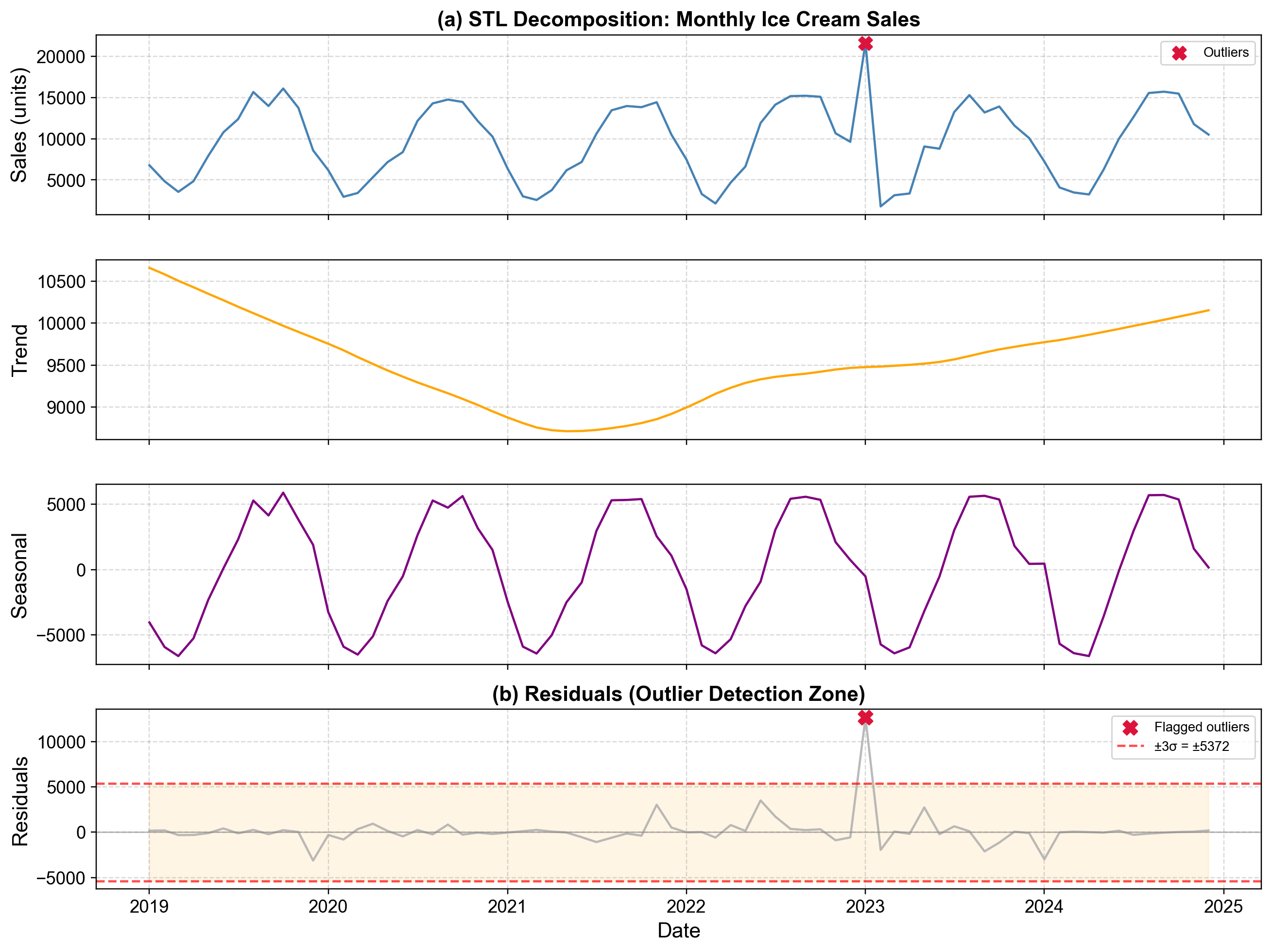
Fig. 5.28 STL decomposition of monthly ice cream sales (2019-2024) with outlier detection applied to residuals. The four panels display the observed series, extracted trend component, seasonal component, and residual component with ±3σ detection bands. January 2023 appears as a dramatic spike in the residual panel, exceeding the upper threshold.

Fig. 5.28 shows the complete STL decomposition revealing how outlier detection benefits from component separation. The top panel displays the observed ice cream sales time series, showing regular summer-winter oscillations with peaks reaching 15,000-16,000 units and valleys dropping to 2,000-4,000 units. January 2023 shows a spike to approximately 21,600 units—high, but not dramatically so compared to typical summer peaks. Without decomposition, we might incorrectly treat this as merely an unusually strong month rather than recognizing it as contextually anomalous.

The second panel displays the extracted trend component, showing smooth long-term movement from approximately 10,700 units in early 2019 to 10,150 units by late 2024. The trend exhibits slight fluctuations but no dramatic jumps, indicating steady underlying demand growth. The STL algorithm’s loess smoothing creates a robust trend estimate that resists contamination from the January 2023 outlier.

The third panel reveals the seasonal component, demonstrating the repeating annual cycle that dominates ice cream sales. Seasonal effects range from approximately -6,400 units in March (late winter) to +5,700 units in August and October (peak summer/early fall). January shows a seasonal component near -530 units in 2023, indicating it’s typically a below-average month. This seasonal estimate remains stable across years, confirming the pattern’s regularity.

The bottom panel displays residuals—the unexplained variation after removing trend and seasonality. Horizontal red dashed lines mark ±3σ thresholds at approximately ±3,900 units. Most residuals cluster tightly between -2,000 and +3,500 units, indicating the trend and seasonal components capture the data structure effectively. However, January 2023 produces a residual near +12,650 units, dramatically exceeding the upper control limit by more than threefold. This spike stands in stark contrast to all other observations, unambiguously identifying it as an anomaly requiring investigation.

Several other observations warrant attention in the residual panel. June 2022 shows a residual near +3,500 units, approaching but not exceeding the threshold—this might represent a legitimate busy period or merit closer examination. July 2022 displays an elevated residual around +1,700 units, suggesting somewhat higher-than-expected sales but within normal variation. November 2021 shows a positive residual around +3,000 units, again elevated but below the threshold. These near-threshold observations demonstrate how we might adjust detection sensitivity: using 2.5σ would flag more observations for review, while 3.5σ would focus only on the most extreme cases.

Interpreting Component Separation:

The power of STL decomposition for outlier detection lies in its ability to answer “unusual compared to what?” The January 2023 value is not unusual compared to the entire dataset range (summer values regularly exceed 15,000), but it is profoundly unusual for January given the strong seasonal pattern. Traditional global threshold methods would miss this contextual anomaly entirely.

Consider what happens without decomposition. Computing a simple global threshold using the entire time series:

• Mean: approximately 9,800 units

• Standard deviation: approximately 4,200 units

• Upper 3σ threshold: 9,800 + 3(4,200) = 22,400 units

The January 2023 value of 21,602 falls below this global threshold, failing to trigger an alarm. The high standard deviation reflects genuine seasonal variation (summer vs. winter sales), diluting the method’s sensitivity to contextual anomalies. STL decomposition solves this by removing systematic variation first, leaving residuals with much lower variance (σ ≈ 1,300) that make genuine anomalies stand out clearly.

Advantages of STL Decomposition

Contextual outlier detection: Automatically adjusts for trend and seasonality, identifying observations that are unusual given their temporal context rather than merely globally extreme Robust estimation: STL’s robust variant uses weighted regression that downweights outliers during trend and seasonal extraction, preventing contamination of the components Visual interpretability: Four-panel decomposition plots clearly show whether variation appears in trend, seasonal, or residual components, facilitating diagnosis Flexible seasonality: Unlike simple seasonal differencing, STL handles complex, slowly changing seasonal patterns and multiple seasonal cycles Diagnostic value: Examining which component contains anomalies reveals the nature of the problem—trend shifts, seasonal disruptions, or isolated residual spikes each suggest different root causes

Practical Considerations

• Parameter Selection: STL decomposition requires specification of smoothing parameters—particularly the seasonal window controlling how much seasonal patterns can vary over time, and the trend window controlling trend smoothness. Default automatic selection works well for many applications, but poor choices can either over-smooth (hiding real changes) or under-smooth (treating variation as structure).

• Additive vs. Multiplicative: The standard STL assumes additive components where seasonal variation magnitude remains constant. When seasonal swings grow proportionally with the level (common in business and economic data), we should log-transform the series before decomposition, then back-transform results. This converts multiplicative patterns to additive ones.

• Threshold Tuning: The 3σ threshold for residuals remains somewhat arbitrary. We should adjust based on application requirements—use 2.5σ for higher sensitivity in critical monitoring applications, or 3.5σ when false positives carry significant investigation costs. Alternatively, consider using the IQR method on residuals for distribution-free thresholding.

• Minimum Data Requirements: STL requires at least two complete seasonal cycles to estimate seasonal components reliably. For monthly data, we need minimum 24 observations, though 3-5 years provides more stable estimates. For data with multiple nested seasonality (e.g., hourly data with both daily and weekly cycles), specialized methods like MSTL may prove more appropriate.

• Computational Efficiency: While STL proves computationally expensive for very long series (millions of observations), modern implementations handle typical business time series (hundreds to thousands of points) efficiently. For real-time monitoring of streaming data, we can refit decomposition periodically rather than with every new observation.

When STL Decomposition Works Best

We should favor STL-based outlier detection when:

• Our data exhibit clear, regular seasonal patterns that we wish to preserve rather than remove

• We need to distinguish between level shifts, seasonal changes, and isolated outliers based on which component shows anomalies

• Visual interpretation matters—stakeholders benefit from seeing trend, seasonal, and residual contributions separately

• The series contains sufficient history (minimum 2-3 seasonal cycles) for reliable component estimation

• We can tolerate slightly higher computational cost compared to simple threshold methods in exchange for better contextual detection

Limitations and Failure Modes

STL decomposition can fail or produce misleading results when:

• Seasonality changes abruptly or irregularly, violating the assumption of smoothly varying seasonal patterns

• The series contains too few cycles for reliable seasonal estimation

• Multiple outliers occur close together, potentially contaminating seasonal or trend estimates despite robustness weighting

• Seasonal patterns exhibit complex interactions with the trend (multiplicative effects) that additive decomposition cannot capture

• Very high-frequency seasonality (daily patterns in minute-level data) creates computational challenges and noise in seasonal estimates

5.6.1.3. Change Point Detection

Change point detection addresses a fundamentally different question than methods we’ve discussed previously. Rather than asking “which observations are outliers?”, we ask “when did the statistical properties of this process fundamentally change?” This distinction proves critical because observations appearing extreme after a change point may actually be normal under the new regime—they’re not outliers to be dismissed but signals of structural transformation requiring investigation [Killick et al., 2012, Truong et al., 2020].

Purpose and Conceptual Framework:

A change point represents a time when one or more statistical properties of a process—typically the mean, variance, or autocorrelation structure—undergo sudden or gradual transition. Unlike isolated outliers that spike briefly then return to baseline, change points persist, creating distinct “before” and “after” regimes. Distinguishing between outliers and change points matters enormously for decision-making: outliers suggest investigating and correcting specific incidents, while change points suggest the system itself has transformed and may require fundamental operational changes.

CUSUM Method:

The Cumulative Sum (CUSUM) control chart provides a widely used approach for detecting mean shifts. We calculate:

(5.14)\[\begin{equation} S_t = \max(0, S_{t-1} + (x_t - \mu_0 - k)) \end{equation}\]

where:

• \(S_t\) is the cumulative sum at time \(t\)

• \(x_t\) is the observation at time \(t\)

• \(\mu_0\) is the target or baseline mean

• \(k\) is the slack parameter (typically 0.5σ to 1σ) allowing tolerance for normal variation

• \(S_0 = 0\) as the starting value

Decision Rule: We flag a change point when \(S_t\) exceeds a threshold \(h\) (commonly 4σ to 5σ). The time when CUSUM first exceeds \(h\) indicates when the sustained shift began. Observations near and after this change point may appear anomalous but actually reflect the new process mean rather than isolated outliers.

Example 5.9

Consider server response time monitoring from January through March 2024:

Baseline period (Day 1-44):

• Mean response time: \(\mu_0 = 195\) ms

• Standard deviation: \(\sigma = 20\) ms

• Response times fluctuate between 150-235 ms with occasional brief spikes

• CUSUM statistic remains below 100, well under detection threshold

Transition period (Day 44-46):

• February 14-16 show extreme response times: 1,048 ms, 1,068 ms, 1,055 ms

• These appear as dramatic outliers, exceeding baseline by 5-fold

• CUSUM accumulates rapidly: 844 → 1,708 → 2,559, crossing threshold around day 45

Post-change regime (Day 47 onward):

• Mean stabilizes at new level: approximately 270 ms (38% increase from baseline)

• Variance increases: σ ≈ 28 ms

• Response times consistently elevated, ranging 230-320 ms

• CUSUM continues accumulating, confirming sustained shift

Interpretation: The three extreme observations (1,048-1,068 ms) are not isolated outliers but rather acute symptoms of an underlying system transition. Treating them as individual anomalies to be filtered would miss the critical insight: the entire system has shifted to a degraded performance state. Investigation should focus on identifying what changed around day 44—perhaps a software deployment, infrastructure modification, or gradual resource exhaustion reaching a tipping point.

Show code cell source

Hide code cell source

import numpy as np

# Simple CUSUM: detect mean shift
baseline_mean = response_times[:30].mean()
baseline_std = response_times[:30].std(ddof=1)

# CUSUM parameters
K = 0.5 * baseline_std
H = 5 * baseline_std
cusum = np.zeros(n)

for t in range(1, n):
    cusum[t] = max(0, cusum[t-1] + (response_times[t] - (baseline_mean + K)))

# Find alarm point
alarm_idx = int(np.argmax(cusum > H)) if (cusum > H).any() else None

Loading ITables v2.6.2 from the init_notebook_mode cell... (need help?)

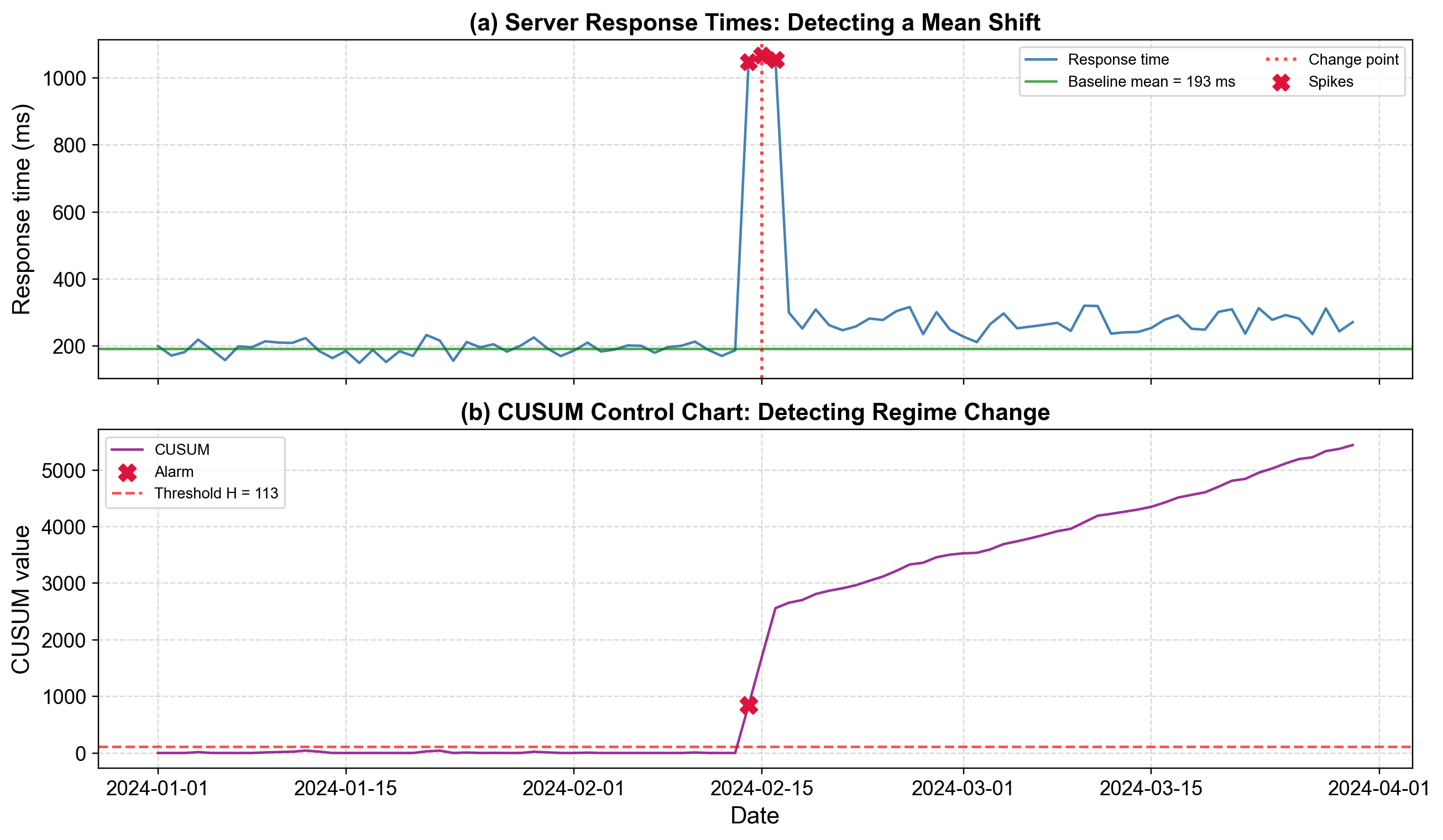
Fig. 5.29 Change point detection using CUSUM on server response times. Panel (a) displays the response time series with baseline mean (green dashed line) and three extreme spikes (red markers) around day 45, followed by sustained elevation. Panel (b) shows the CUSUM statistic accumulating gradually until day 45, then rapidly crossing the threshold (red line), confirming a regime shift rather than isolated outliers.

The figure illustrates how change point detection distinguishes regime shifts from isolated anomalies. Panel (a) shows server response times measured daily from January through March 2024. During days 1-44, response times exhibit stable behavior around 195 ms (green dashed line) with typical variation between 150-235 ms. The pattern appears consistent with a well-functioning system experiencing normal load fluctuations.

Days 44-46 (February 14-16) show dramatic spikes reaching approximately 1,050 ms—marked with red circles as extreme observations. A naive outlier detection approach would flag these three points, investigate them individually, then move on. However, the subsequent pattern reveals a more serious problem: even after the extreme spikes subside, response times never return to baseline. From day 47 onward, the “new normal” stabilizes around 270 ms—consistently 70-80 ms higher than the historical baseline. This elevated performance persists through the remainder of the observation period, indicating permanent degradation rather than transient disruption.

Panel (b) displays the CUSUM statistic, which accumulates positive deviations from the baseline mean. During the stable period (days 1-44), CUSUM fluctuates between 0 and 50, occasionally rising when response times exceed baseline but resetting when they fall below. This behavior indicates normal variation—brief excursions above mean are balanced by returns below mean, producing no sustained trend in the cumulative sum.

The pattern changes dramatically at day 44. The CUSUM begins accelerating upward, reaching approximately 850 by day 45, 1,700 by day 46, and 2,550 by day 47—well exceeding the detection threshold (red horizontal line) around 500. Critically, the CUSUM continues accumulating after the extreme spikes end, reaching approximately 5,400 by day 90. This sustained accumulation despite the absence of dramatic spikes confirms that we’re observing a permanent shift in mean performance, not merely isolated outliers.

Distinguishing Outliers from Change Points:

The server response time example highlights the key distinction:

Isolated outliers:

• Spike dramatically above (or below) baseline

• Quickly return to previous normal levels

• CUSUM accumulates briefly but resets as normal observations follow

• Appropriate response: Investigate specific incident, correct if error, accept if legitimate extreme

Change points:

• May include extreme transitional observations

• New level persists after initial transition

• CUSUM accumulates continuously, never resetting

• Appropriate response: Investigate what changed in the system, decide whether to accept new regime or intervene to restore baseline

In our example, treating the 1,050 ms observations as outliers to be removed would leave the fundamental problem unaddressed. The real issue isn’t three bad measurements but rather a system that has degraded from 195 ms to 270 ms average response time—a 38% performance loss that will compound into significant user experience deterioration and potential capacity problems.

Advantages of Change Point Detection

Regime identification: Separates structural changes from random variation, preventing misclassification of new-normal behavior as outliers Early warning: Detects emerging shifts before they become obvious, enabling proactive intervention Reduced false positives: Prevents repeated flagging of observations that are normal under the new regime Root cause focus: Directs attention to “what changed in the system?” rather than “which observations are weird?” Quantifies timing: Identifies when transitions occurred, facilitating correlation with operational events (deployments, configuration changes, hardware failures)

Method Variations and Extensions

Two-sided CUSUM: The formulation above detects upward shifts only. For complete monitoring, we should run parallel downward CUSUM:

\[\begin{equation*} S_t^- = \max(0, S_{t-1}^- - (x_t - \mu_0 + k)) \end{equation*}\]

This detects both performance degradation (upward shift in response time) and unusual improvements (downward shift) that might indicate measurement errors or undocumented system changes.

Bayesian Change Point Detection: Methods like the Bayesian online change point detection algorithm estimate the posterior probability distribution over change point locations, providing uncertainty quantification rather than single-point estimates. This proves valuable when we need to assess confidence in detected changes.

Multiple Change Points: Real systems often undergo multiple regime shifts. We can apply methods like Pruned Exact Linear Time (PELT) or Binary Segmentation to partition a long series into multiple homogeneous segments, identifying all significant change points simultaneously.

Variance Change Detection: CUSUM focuses on mean shifts. When variance changes matter (detecting periods of increased volatility), we should use specialized methods like GARCH models or the running variance control chart.

Practical Implementation Guidance

Parameter Selection:

• Slack parameter (k): Typically set to 0.5σ to 1.0σ. Smaller values increase sensitivity but raise false positive rates. We should tune based on the magnitude of shift we wish to detect—use 0.5σ for detecting small shifts (~1σ), 1.0σ for detecting larger shifts (~2σ).

• Threshold (h): Common values range from 4σ to 5σ. Higher thresholds reduce false alarms but increase detection delay. We can use Average Run Length (ARL) theory to select thresholds achieving desired false alarm rates under stable conditions.

Baseline Establishment:

We must establish \(\mu_0\) and \(\sigma\) from a stable historical period. If the initial data already contain change points or outliers, parameter estimates become biased and detection performance suffers. Consider using robust estimates (median, MAD) or manually selecting a known-stable baseline period.

Real-Time vs. Retrospective:

CUSUM works online—we can update it with each new observation for real-time monitoring. For retrospective analysis of historical data where we suspect multiple change points, batch methods like PELT often provide better segmentation.

Post-Detection Actions:

When CUSUM signals a change point:

1. Correlate with events: Check logs, deployment schedules, infrastructure changes around the detected time

2. Characterize the shift: Quantify new mean/variance, assess operational impact

3. Decide on response: Accept new regime, intervene to restore baseline, or escalate for investigation

4. Reset monitoring: After confirming a permanent change, reset CUSUM with new baseline parameters to detect subsequent shifts

When Change Point Detection Works Best

We should apply change point methods when:

• Our monitoring objective includes detecting system state changes, not just anomalous observations

• The process can undergo sudden or gradual regime shifts due to operational changes, degradation, or external factors

• We need to distinguish between “system working as designed with occasional spikes” versus “system has fundamentally changed”

• Historical context matters—we want to know when things changed, not merely that they’re currently unusual

• False positives carry lower cost than missed regime shifts (in critical infrastructure monitoring)

Limitations and Failure Modes

Change point detection faces challenges when:

• Multiple change points occur in close succession, making individual transitions hard to isolate

• Changes occur gradually rather than abruptly, producing weak signals that CUSUM accumulates slowly

• High baseline variance makes small-to-moderate shifts difficult to detect above noise

• Seasonal patterns or trends complicate baseline definition—we should detrend or deseasonalize first

• The “change” is temporary (a week-long elevated period) rather than permanent, potentially triggering false alarms