Remark

Please be aware that these lecture notes are accessible online in an ‘early access’ format. They are actively being developed, and certain sections will be further enriched to provide a comprehensive understanding of the subject matter.

2.3. Handling Missing Values

After identifying missing values in a dataset, addressing them effectively is essential to ensure the accuracy and reliability of analyses. Missing data can introduce bias, reduce statistical power, and impact the validity of results. Below is a detailed guide to various methods for handling missing values. Note that we can only explain a subset of these methods at this stage. Some advanced techniques, particularly those requiring familiarity with time series modeling methods.

2.3.1. Deletion Methods

When addressing missing data, listwise deletion and pairwise deletion are two foundational methods commonly used in data analysis. These approaches are straightforward to implement but vary in their impact on the dataset and the potential biases they introduce. Below, we explain these methods in detail, incorporating examples and highlighting their strengths and limitations.

2.3.1.1. Listwise Deletion

Listwise deletion, also known as casewise deletion, involves removing any observation (row) that contains missing values in one or more variables. This results in a reduced dataset that includes only complete cases. While this method ensures consistency across analyses, it can lead to significant data loss if missingness is widespread.

• In machine learning, listwise deletion is often used in ranking tasks where incomplete observations can distort model predictions [Li et al., 2024].

• In time-series analysis, listwise deletion ensures that only complete records are used for modeling trends or patterns.

However, listwise deletion can lead to biased results if the missing data are not Missing Completely At Random (MCAR).

2.3.1.2. Pairwise Deletion

Pairwise deletion takes a more flexible approach by removing only the specific variables or pairs of variables that contain missing values while retaining all other observations. This allows for more data to be preserved compared to listwise deletion. It is particularly useful for analyses involving relationships between variables (e.g., correlations or covariances), where not all variables need to be analyzed simultaneously.

• Pairwise deletion is especially effective when working with complex data structures like networks or sparse datasets [Wilcox et al., 2023].

• In image-text retrieval tasks, pairwise deletion has been used alongside listwise ranking methods to improve retrieval performance by leveraging complementary strengths [Li et al., 2024].

Despite its advantages, pairwise deletion can still lead to biased results if the missing data are not Missing At Random (MAR) or MCAR. Additionally, sample sizes may vary across analyses depending on which variables are included, potentially complicating interpretation.

2.3.1.3. Example: Demonstrating Listwise and Pairwise Deletion

This dataset contains daily temperature records for Columbia, Missouri, spanning from October 1 to October 10, 2024. The temperatures are presented in both standard and metric units. The data was collected by the University of Missouri weather station and sourced from the National Centers for Environmental Information (NCEI), a division of NOAA. You can access the original data source here: NCEI Climate Data.

Note

This dataset is intended for educational use only. Although based on historical data, it has been modified for training purposes to illustrate techniques for handling missing data in Python and may not be suitable for operational weather analysis or forecasting. Here, TMIN stands for minimum daily temperature (in degrees farenhight) and TMAX stands for maximum daily temperature (in degrees farenhight).

Table 2.2 Climate Dataset with Missing Values

	TMIN	TMAX
2024-10-01	49.0	72.0
2024-10-02	44.0	74.0
2024-10-03	56.0	87.0
2024-10-04	NaN	NaN
2024-10-05	62.0	89.0
2024-10-06	NaN	79.0
2024-10-07	47.0	72.0
2024-10-08	43.0	NaN
2024-10-09	46.0	78.0
2024-10-10	49.0	80.0

This dataset contains missing values (NaN) in various rows and columns. It can be visualized as follows. Fig. 2.1 highlights missing cells in red and non-missing cells in green.

Fig. 2.1 Visualization of Table 2.2, where green shades show entries without missing values and orange cells show entries with missing values.

In listwise deletion, rows with any missing values are removed entirely before performing analyses. This ensures that only complete cases are retained.

Show code cell source

Hide code cell source

import pandas as pd
df = pd.read_csv('chapter02_data/data_10day_standard_missing.csv', index_col=0)
print('\nData:')
display(df)

# Apply listwise deletion
df_listwise = df.dropna(how='any')
print('\nAfter listwise deletion:')
display(df_listwise)

Data:

	TMIN	TMAX
10/1/24	49.0	72.0
10/2/24	44.0	74.0
10/3/24	56.0	87.0
10/4/24	NaN	NaN
10/5/24	62.0	89.0
10/6/24	NaN	79.0
10/7/24	47.0	72.0
10/8/24	43.0	NaN
10/9/24	46.0	78.0
10/10/24	49.0	80.0

After listwise deletion:

	TMIN	TMAX
10/1/24	49.0	72.0
10/2/24	44.0	74.0
10/3/24	56.0	87.0
10/5/24	62.0	89.0
10/7/24	47.0	72.0
10/9/24	46.0	78.0
10/10/24	49.0	80.0

As shown above, rows 0, 1, 2, 4, 5, and 6 are removed because they contain at least one missing value. Only rows 3 and 7 remain in the dataset after applying listwise deletion.

In some analyses, such as calculating means or correlations, we may want to utilize all available data for specific variables rather than discarding entire rows. Pairwise deletion allows us to calculate statistics independently for each variable by ignoring NaN values.

Show code cell source

Hide code cell source

# Calculate mean using pairwise deletion (mean of each column ignoring NaN values)
pairwise_mean = df.mean(skipna=True).round(3)
print("Pairwise Mean:")
print(pairwise_mean)

# Calculate mean using listwise deletion (on the reduced dataset)
listwise_mean = df_listwise.mean(skipna=True).round(3)
print("\nListwise Mean:")
print(listwise_mean)

Pairwise Mean:
TMIN    49.500
TMAX    78.875
dtype: float64

Listwise Mean:
TMIN    50.429
TMAX    78.857
dtype: float64

• Pairwise mean uses all available pairs for each variable (maximizing data).

• Listwise mean uses only completely observed rows (more data loss).

2.3.1.4. Conclusion

Table 2.3 Combined Advantages and Disadvantages of Listwise vs Pairwise Deletion

Feature	Listwise Deletion	Pairwise Deletion
Data Retention	Removes entire rows with missing data, leading to significant data loss if missingness is widespread.	Retains more data by analyzing specific columns independently, minimizing overall data loss.
Bias Risk	High risk of bias if missing data are not Missing Completely At Random (MCAR), as certain groups may be disproportionately excluded.	Lower bias risk compared to listwise deletion but still present if data are not Missing At Random (MAR) or MCAR.
Ease of Use	Simple to implement and interpret, requiring minimal computational effort.	More complex implementation; requires careful handling to ensure valid comparisons across analyses.
Consistency Across Analyses	Ensures consistency by using the same subset of complete cases for all analyses.	Sample size varies across analyses depending on the variables involved, potentially complicating interpretation.
Applicability	Suitable for datasets with minimal missingness or when consistency across analyses is critical.	Useful for preserving data in exploratory analyses or when relationships between specific variables are the focus.

Key Considerations for Deletion Methods

Listwise Deletion:

• Best suited for:

  • Datasets with minimal missing values (<5% missingness)

  • Analyses requiring consistent sample sizes

  • Cases where missing data are MCAR

• Primary advantages:

  • Simplicity in implementation

  • Consistency across analyses

  • Unbiased parameter estimates when MCAR assumption holds

Pairwise Deletion:

• Best suited for:

  • Exploratory data analysis

  • Computing correlation matrices

  • Cases where maximizing available data is crucial

• Primary advantages:

  • Preserves more information

  • More efficient use of available data

  • Reduced bias compared to listwise deletion

Implementation Guidelines

1. Before Applying Deletion Methods:

   • Assess the pattern and extent of missingness

   • Verify MCAR assumption if possible

   • Consider the impact on sample size

2. When Choosing Between Methods:

   • Use listwise deletion when:

     • Missing data are MCAR

     • Sample size remains adequate after deletion

     • Consistent sample size is required

   • Use pairwise deletion when:

     • Maximizing available information is crucial

     • Different analyses can tolerate varying sample sizes

     • Preliminary or exploratory analyses are being conducted

The choice between listwise and pairwise deletion should be guided by:

1. The research objectives

2. The missing data mechanism (MCAR, MAR, or MNAR)

3. The proportion of missing values

4. The importance of maintaining consistent sample sizes across analyses

Both methods have their place in data analysis, but neither should be applied without careful consideration of their assumptions and potential impact on the results. When possible, more sophisticated methods like multiple imputation might be more appropriate for handling missing data, especially when the missingness mechanism is not MCAR or when the proportion of missing data is substantial.

2.3.2. Simple Imputation Methods

Simple imputation methods represent a fundamental approach to handling missing values in datasets. These methods replace missing values with estimated values based on various simple rules or calculations. While more sophisticated techniques exist, simple imputation methods remain popular due to their ease of implementation, computational efficiency, and interpretability.

These methods can be broadly categorized into two groups:

1. Value Substitution Methods: These methods replace missing values with a calculated statistic (like mean or median) or a predefined constant value. They are straightforward to implement and understand but may not capture the temporal dynamics of the data.

2. Sequential Methods: These approaches leverage the ordered nature of data, particularly useful in time series. They include methods like Last Observation Carried Forward (LOCF) and Next Observation Carried Backward (NOCB), which use neighboring values to fill gaps.

While these methods are computationally efficient and easy to implement, they each come with their own assumptions and limitations. The choice of method should be guided by the nature of the data, the pattern of missingness, and the requirements of subsequent analyses.

2.3.2.1. Simple Value Substitution Methods

One of the most straightforward approaches to handling missing values is through simple value substitution. These methods include mean imputation, median imputation, and constant value imputation, each replacing missing values with a specific type of value.

Consider the dataset from Fig. 2.1 with missing values:

These methods work as follows:

1. Mean Imputation: Replaces missing values with the average of the available data. This method is particularly useful for normally distributed variables and large datasets.

2. Median Imputation: Uses the median value of the available data, making it more robust to outliers and suitable for skewed distributions.

3. Constant Value Imputation: Replaces missing values with a predefined constant (often zero), useful when missing values have a specific meaning in the context.

In Fig. 2.2, missing values in each column are replaced with the mean value calculated from the available data in that column. The animation demonstrates how each NaN value is systematically replaced with the column’s mean, preserving the central tendency of the dataset while potentially reducing variability.

Fig. 2.2 Visualization of Mean Imputation. Missing values in each column are replaced with the mean value of that column.

For column TMIN, the mean is:

\[\text{Mean}_{TMIN} = 49.5\]

For column TMAX, the mean is:

\[\text{Mean}_{TMAX} = 78.875\]

Mean-imputed data:

Date	TMIN	TMAX
10/1/24	49.0	72.0
10/2/24	44.0	74.0
10/3/24	56.0	87.0
10/4/24	49.5	78.9
10/5/24	62.0	89.0
10/6/24	49.5	79.0
10/7/24	47.0	72.0
10/8/24	43.0	78.9
10/9/24	46.0	78.0
10/10/24	49.0	80.0

In Fig. 2.3, missing values are imputed with the median of the respective column. Because medians rely on ordered values rather than averages, this method is less affected by outliers compared to mean imputation.

Fig. 2.3 Visualization of Median Imputation. Missing values in each column are replaced with the median value of that column.

For column TMIN, the median is:

\[\text{Median}_{TMIN} = 48.0\]

For column TMAX, the median is:

\[\text{Median}_{TMAX} = 78.5\]

Median-imputed data:

Date	TMIN	TMAX
10/1/24	49.0	72.0
10/2/24	44.0	74.0
10/3/24	56.0	87.0
10/4/24	48.0	78.5
10/5/24	62.0	89.0
10/6/24	48.0	79.0
10/7/24	47.0	72.0
10/8/24	43.0	78.5
10/9/24	46.0	78.0
10/10/24	49.0	80.0

In Fig. 2.4, missing values are imputed using a constant value. Here, missing entries are replaced with 0, which might be appropriate if missingness represents “no observation” or an absence of measurement, though it can strongly distort the dataset’s distribution.

Fig. 2.4 Visualization of Constant Value Imputation. Missing values in each column are replaced with a constant value (e.g., zero).

For constant value imputation:

\[\text{Missing Value} = c, \quad c = 0\]

Constant-value (zero) imputed data:

Date	TMIN	TMAX
10/1/24	49.0	72.0
10/2/24	44.0	74.0
10/3/24	56.0	87.0
10/4/24	0.0	0.0
10/5/24	62.0	89.0
10/6/24	0.0	79.0
10/7/24	47.0	72.0
10/8/24	43.0	0.0
10/9/24	46.0	78.0
10/10/24	49.0	80.0

These methods can be easily implemented in Python using pandas:

Show code cell source

Hide code cell source

import pandas as pd

# Load the dataset
df = pd.read_csv('chapter02_data/data_10day_standard_missing.csv', index_col=0)
print("\nData:")
display(df)

# Mean imputation
col_means = df.mean(axis=0, skipna=True)
print("\nColumn Means:")
print(col_means)
mean_imputed = df.fillna(col_means)
print("\nMean Imputed Data:")
display(mean_imputed)

# Median imputation
col_medians = df.median(axis=0, skipna=True)
print("\nColumn Medians:")
print(col_medians)
median_imputed = df.fillna(col_medians)
print("\nMedian Imputed Data:")
display(median_imputed)

# Constant value imputation (e.g., replace with zero)
constant_imputed = df.fillna(0)
print("\nConstant Value Imputed Data:")
display(constant_imputed)

Data:

	TMIN	TMAX
10/1/24	49.0	72.0
10/2/24	44.0	74.0
10/3/24	56.0	87.0
10/4/24	NaN	NaN
10/5/24	62.0	89.0
10/6/24	NaN	79.0
10/7/24	47.0	72.0
10/8/24	43.0	NaN
10/9/24	46.0	78.0
10/10/24	49.0	80.0

Column Means:
TMIN    49.500
TMAX    78.875
dtype: float64

Mean Imputed Data:

	TMIN	TMAX
10/1/24	49.0	72.000
10/2/24	44.0	74.000
10/3/24	56.0	87.000
10/4/24	49.5	78.875
10/5/24	62.0	89.000
10/6/24	49.5	79.000
10/7/24	47.0	72.000
10/8/24	43.0	78.875
10/9/24	46.0	78.000
10/10/24	49.0	80.000

Column Medians:
TMIN    48.0
TMAX    78.5
dtype: float64

Median Imputed Data:

	TMIN	TMAX
10/1/24	49.0	72.0
10/2/24	44.0	74.0
10/3/24	56.0	87.0
10/4/24	48.0	78.5
10/5/24	62.0	89.0
10/6/24	48.0	79.0
10/7/24	47.0	72.0
10/8/24	43.0	78.5
10/9/24	46.0	78.0
10/10/24	49.0	80.0

Constant Value Imputed Data:

	TMIN	TMAX
10/1/24	49.0	72.0
10/2/24	44.0	74.0
10/3/24	56.0	87.0
10/4/24	0.0	0.0
10/5/24	62.0	89.0
10/6/24	0.0	79.0
10/7/24	47.0	72.0
10/8/24	43.0	0.0
10/9/24	46.0	78.0
10/10/24	49.0	80.0

Table 2.4 Advantages and Disadvantages of Simple Value Substitution Methods for Time Series

Method	Advantages	Disadvantages
Mean Imputation	- Simple to implement and understand - Preserves the overall mean of the variable - Computationally efficient - Suitable for large datasets with stationary behavior	- Breaks temporal dependence structure - Ignores seasonality and trends - Can create flat segments, reducing variability - Sensitive to outliers - May lead to biased autocorrelation estimates
Median Imputation	- Robust to outliers - Suitable for skewed distributions - Preserves median of the variable - Less sensitive to extreme values	- Does not account for time order - Ignores seasonality and cyclic patterns - Can distort lag relationships - Creates unrealistic continuity in temporal context - May affect variance structure
Constant Value	- Simple and quick to apply - Useful when missing values indicate a specific state (e.g., sensor failure) - Preserves interpretability in some contexts	- Completely ignores temporal dynamics - May introduce artificial level shifts - Creates unrealistic patterns for continuous processes - Can distort trend and seasonality modeling - May bias autocorrelation and forecast models

Implementation Guidelines for Time Series

When applying these methods to time series, consider:

1. Temporal Structure:

   • Avoid using simple imputation for long gaps as it disrupts autocorrelation

   • Prefer methods that account for seasonality and trends (e.g., interpolation) when feasible

   • For stationary series with minimal variation, mean or median may be less harmful but still limited

2. Data Quality Checks:

   • Assess autocorrelation function (ACF) and partial autocorrelation function (PACF) before and after imputation

   • Examine residual patterns to detect artificial flattening

   • Compare imputed values against seasonal averages when applicable

3. Documentation:

   • Record the chosen method, justification, and temporal considerations

   • Document the proportion and location of imputed points (isolated vs. block missingness)

   • Note any limitations for downstream time series models (ARIMA, LSTM, etc.)

These simple imputation methods are generally discouraged for time series because they ignore temporal dependence, seasonality, and trend structures. They can lead to biased parameter estimates and poor forecasting performance. Use them only for exploratory analysis or when missingness is minimal and random.

2.3.2.2. Last Observation Carried Forward (LOCF)

Last Observation Carried Forward (LOCF) is a widely used method for handling missing data in longitudinal studies, clinical trials, and time-series analysis[Bourke et al., 2020, Jørgensen et al., 2014]. This technique involves replacing missing values with the most recently observed value, which is then propagated forward to fill subsequent gaps[Bourke et al., 2020, Jørgensen et al., 2014]. LOCF operates under the assumption that the last known observation serves as a reasonable proxy for subsequent missing values.

LOCF is particularly well-suited for time-series data where trends are expected to exhibit continuity or stability, such as weather patterns, stock prices, or medical monitoring. However, it’s crucial to note that LOCF has limitations that warrant careful consideration before implementation.

To illustrate the LOCF method, consider the following synthetic time-series dataset containing missing values:

Table 2.5 Synthetic Time Series Dataset with Missing Values

Date	TMIN	TMAX	PERCIP
2025-01-01	1.0	NaN	1.0
2025-01-02	2.0	2.0	NaN
2025-01-03	NaN	3.0	3.0
2025-01-04	4.0	4.0	4.0
2025-01-05	5.0	NaN	5.0
2025-01-06	NaN	6.0	6.0
2025-01-07	7.0	7.0	NaN
2025-01-08	8.0	8.0	8.0

In Table 2.5, TMIN represents ‘Daily Minimum Temperature (°C)’, TMAX denotes ‘Daily Maximum Temperature (°C)’, and PERCIP stands for ‘Daily Accumulated Precipitation’. Before applying LOCF, it’s important to understand the pattern and distribution of missing values in our dataset.

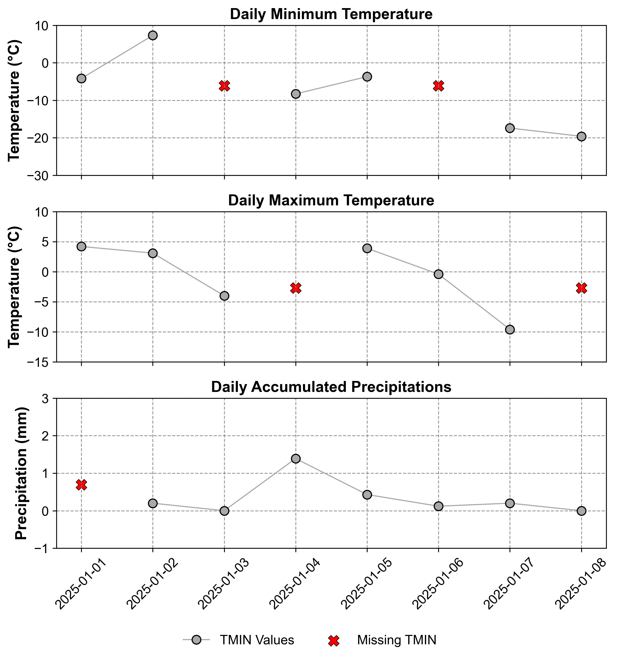
Fig. 2.5 Time series corresponding to Table 2.5. The top panel shows Daily Minimum Temperature (°C), the middle panel displays Daily Maximum Temperature (°C), and the bottom panel illustrates Daily Accumulated Precipitation. Missing points are visualized using an ‘x’ sign in each panel.

Fig. 2.5 reveals the temporal pattern of missing values across our three variables. We can observe that:

• TMIN (top panel) has gaps on January 3rd and 6th

• TMAX (middle panel) shows missing values on January 1st and 5th

• PERCIP (bottom panel) has missing data on January 2nd and 7th

This visualization helps us understand how LOCF will propagate values forward to fill these gaps. The following animation demonstrates the LOCF process:

Fig. 2.6 Visualization of Last Observation Carried Forward (LOCF) Imputation. Missing values are filled using the last observed value in each column.

In Fig. 2.6, we can see how LOCF systematically fills each missing value with its most recent observed value. For example:

• When TMIN is missing on January 3rd, it’s filled with the value from January 2nd

• The missing TMAX value on January 5th is replaced with the January 4th observation

• For PERCIP, the January 2nd gap is filled using the January 1st value

Remark

A key limitation of LOCF arises when missing values occur at the beginning of the dataset. In such instances, there is no prior observation to carry forward, rendering LOCF ineffective. Consequently, these initial missing values remain as NaN and require alternative imputation methods.

Show code cell source

Hide code cell source

import pandas as pd

# Load the dataset
df = pd.read_csv('chapter02_data/generated_sample_time_series_climate.csv', index_col=0)

# LOCF imputation
locf_imputed = df.ffill()
print("\nLast Observation Carried Forward (LOCF) Imputed Data:")
display(locf_imputed)

Last Observation Carried Forward (LOCF) Imputed Data:

	TMIN	TMAX	PERCIP
Date
2025-01-01	-4.2	4.2	NaN
2025-01-02	7.3	3.1	0.20
2025-01-03	7.3	-4.0	0.00
2025-01-04	-8.3	-4.0	1.39
2025-01-05	-3.7	3.9	0.43
2025-01-06	-3.7	-0.4	0.12
2025-01-07	-17.4	-9.6	0.20
2025-01-08	-19.6	-9.6	0.00

Explanation:

The Last Observation Carried Forward (LOCF) method has been applied to our synthetic time-series dataset, yielding the following results:

1. Column TMIN (Daily Minimum Temperature):

   • The missing value on 2025-01-03 is imputed with 7.3°C, which is carried forward from the last observed value on 2025-01-02.

   • Similarly, the gap at 2025-01-06 is filled with -3.7°C, using the most recent observation from 2025-01-05.

2. Column TMAX (Daily Maximum Temperature):

   • For the missing data point on 2025-01-04, LOCF assigns -4.0°C, based on the previous day’s reading.

   • The final missing value on 2025-01-08 is imputed as -9.6°C, carried forward from 2025-01-07.

3. Column PERCIP (Daily Accumulated Precipitation):

   • Notably, the missing value at the dataset’s start (2025-01-01) remains unfilled, as LOCF cannot impute when there’s no prior observation.

This imputation process ensures continuity in the time series by propagating the last known values forward to fill gaps, maintaining the dataset’s temporal structure.

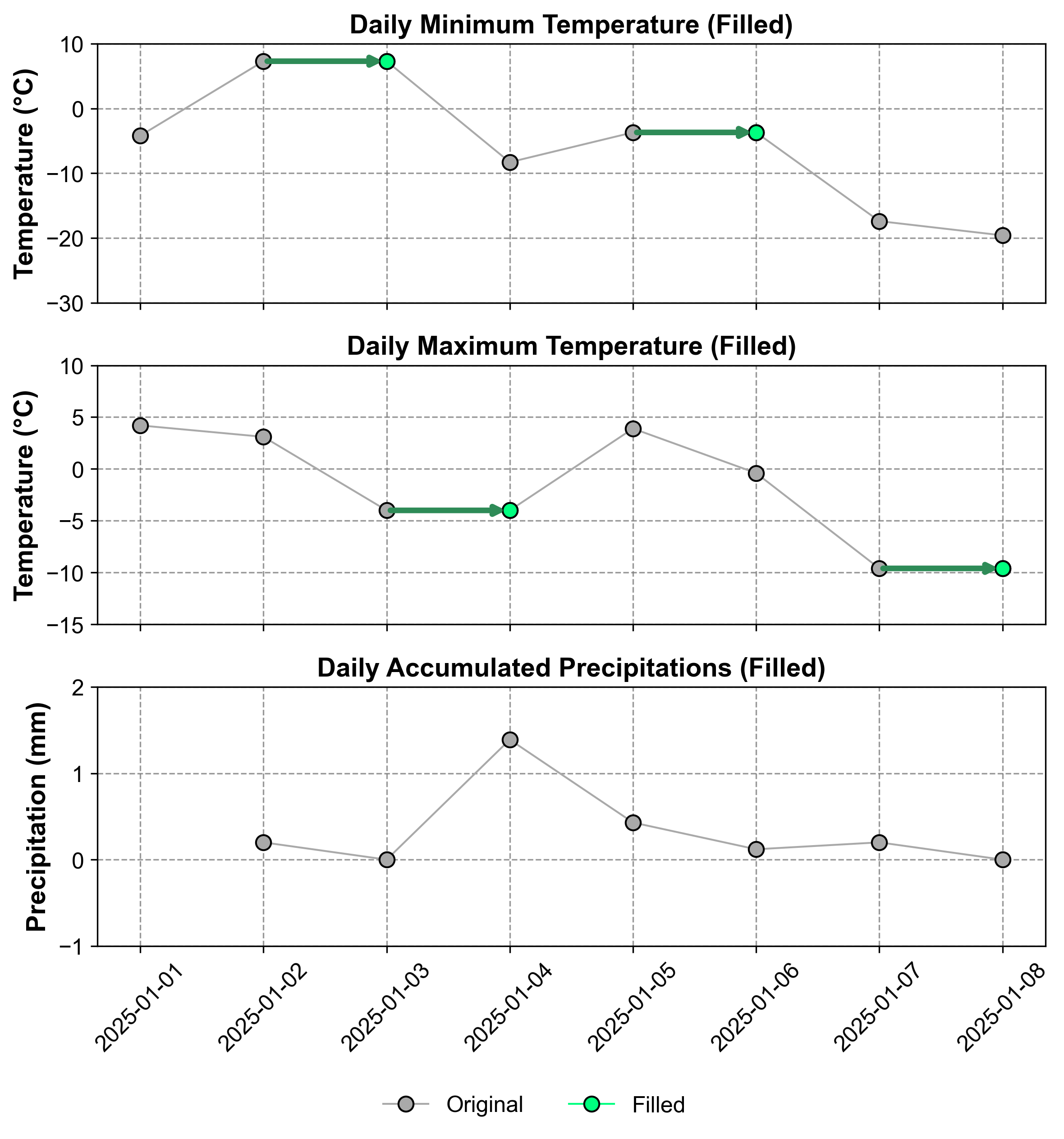
Fig. 2.7 Visualization of the time series after LOCF imputation. Gray points represent original values, while green points indicate imputed values using the forward-fill method.

Fig. 2.7 illustrates the impact of LOCF on our dataset. Original data points are shown in gray, while the imputed values are highlighted in green. This visual representation helps to understand how LOCF maintains the trend of the last observed value until new data becomes available, potentially creating step-like patterns in the imputed series.

2.3.2.3. Next Observation Carried Backward (NOCB)

The Next Observation Carried Backward (NOCB) method is a missing value recovery technique that fills in missing values using the next observed value after the gap. This approach assumes that future observations can reasonably inform earlier gaps, making it particularly suitable for time-series data where trends or patterns are expected to remain stable over time.

NOCB is commonly applied in fields such as healthcare, sustainability research, and time-series modeling. For example:

• In healthcare, NOCB is used to fill gaps in physiological state variables by assuming that future test results can reflect earlier states [Hecker et al., 2022].

• In sustainability research, baseline values of new participants are often replaced with their values at first follow-up using NOCB [Hecker et al., 2022].

Using the same dataset from our LOCF example, we can visualize how NOCB fills missing values by looking forward in time. For our temperature and precipitation data:

• A missing TMIN value on January 3rd would be filled using the value from January 4th

• The missing TMAX value on January 1st would be replaced with the January 2nd observation

• For PERCIP, the January 2nd gap would be filled using the January 3rd measurement

The following animation demonstrates this backward filling process:

Fig. 2.8 Visualization of Next Observation Carried Backward (NOCB) Imputation. Missing values are filled using the next observed value in each column.

In Fig. 2.8, we can observe how:

• The imputation process starts from the end of the time series and moves backward

• Each missing value is replaced with the next available observation in its column

• The method preserves the temporal patterns within each variable independently

• Missing values at the end of the series remain unfilled due to the absence of future observations

• The process continues until all possible gaps are filled, except those at the end of the dataset

Remark

If a missing value occurs at the end of the dataset, there is no subsequent observation to carry backward, and it remains as NaN.

Python Implementation:

Show code cell source

Hide code cell source

# NOCB imputation
nocb_imputed = df.bfill()
print("\nNext Observation Carried Backward (NOCB) Imputed Data:")
display(nocb_imputed)

Next Observation Carried Backward (NOCB) Imputed Data:

	TMIN	TMAX	PERCIP
Date
2025-01-01	-4.2	4.2	0.20
2025-01-02	7.3	3.1	0.20
2025-01-03	-8.3	-4.0	0.00
2025-01-04	-8.3	3.9	1.39
2025-01-05	-3.7	3.9	0.43
2025-01-06	-17.4	-0.4	0.12
2025-01-07	-17.4	-9.6	0.20
2025-01-08	-19.6	NaN	0.00

Explanation:

The Next Observation Carried Backward (NOCB) method has been applied to our synthetic time-series dataset, yielding the following results:

1. Column TMIN (Daily Minimum Temperature):

   • The missing value on 2025-01-03 is imputed with -8.3°C, which is carried backward from the next observed value on 2025-01-04.

   • Similarly, the gap at 2025-01-06 is filled with -17.4°C, using the subsequent observation from 2025-01-07.

2. Column TMAX (Daily Maximum Temperature):

   • For the missing data point on 2025-01-04, NOCB assigns -0.4°C, based on the next day’s reading.

   • Notably, the final missing value on 2025-01-08 remains unfilled, as there are no subsequent observations to carry backward.

3. Column PERCIP (Daily Accumulated Precipitation):

   • The missing value at the dataset’s start (2025-01-01) is imputed as 0.2, carried backward from the next available observation.

This imputation process ensures continuity in the time series by propagating future known values backward to fill gaps, maintaining the dataset’s temporal structure.

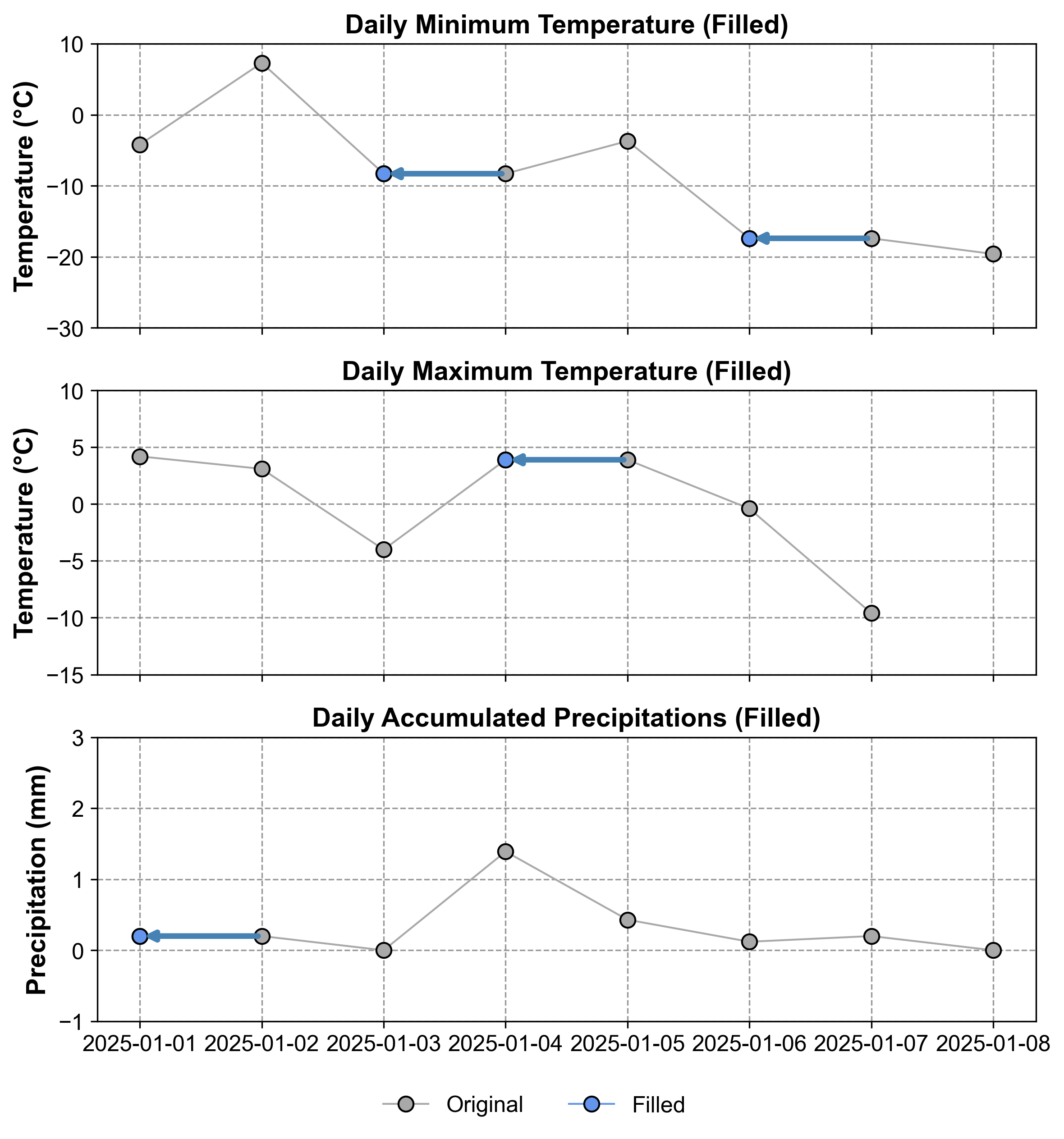
Fig. 2.9 Visualization of the time series after NOCB imputation. Gray points represent original values, while blue points indicate imputed values using the backward-fill method.

Fig. 2.9 illustrates the impact of NOCB on our dataset. Original data points are shown in gray, while the imputed values are highlighted in blue. This visual representation helps to understand how NOCB maintains the trend of the next observed value, filling gaps with future information. This approach can create step-like patterns in the imputed series, but in the opposite direction compared to LOCF.

2.3.2.4. Comparison of LOCF and NOCB

The following table summarizes the key differences between Last Observation Carried Forward (LOCF) and Next Observation Carried Backward (NOCB):

Table 2.6 Comparison of LOCF and NOCB Imputation Methods

Feature	LOCF	NOCB
Direction of Imputation	Fills gaps using the last observed value before the gap	Fills gaps using the next observed value after the gap
Unfilled Values	Missing values at the start of the dataset remain unfilled	Missing values at the end of the dataset remain unfilled
Assumptions	Assumes continuity or stability over time	Assumes future observations can inform earlier gaps
Bias Risk	Can introduce bias if trends change significantly after the last observed value	Can introduce bias if trends change significantly before the next observed value
Uncertainty Handling	Does not account for uncertainty in imputation, leading to overly narrow confidence intervals	Similar to LOCF, does not account for uncertainty in imputation
Applicability	Useful for time-series data where past trends influence future observations	Useful for time-series data where future trends can inform earlier gaps

When choosing between LOCF and NOCB methods, it’s important to understand their respective strengths and limitations. Let’s first examine their key advantages:

Advantages of LOCF and NOCB

Advantages of LOCF:

1. Simplicity: Easy to implement and computationally efficient.

2. Preserves Dataset Size: Retains all rows in the dataset by imputing missing values instead of removing them.

3. Applicability to Time-Series Data: Works well when past observations are expected to influence future ones.

Advantages of NOCB:

1. Reverse Imputation Direction: Fills missing values by looking forward in time, making it effective for datasets where future trends are more reliable indicators than past trends.

2. Preserves Dataset Size: Like LOCF, it retains all rows by imputing missing values.

While these advantages make both methods attractive for their simplicity and practical implementation, they also come with several important limitations that should be carefully considered:

Limitations of LOCF and NOCB

Limitations of LOCF:

1. Bias Introduction:

• Assumes that missing final values are identical to the last recorded values, which may not always be plausible [Jørgensen et al., 2014].

• For example, in weight loss studies, carrying forward a participant’s last recorded weight might underestimate actual weight loss [Bourke et al., 2020].

2. Narrow Confidence Intervals:

• Does not account for uncertainty introduced by imputation, leading to overly narrow confidence intervals [Jørgensen et al., 2014].

3. Conservative Estimates:

• Only considers the last observed value, ignoring potential changes or trends in the outcome variable over time [Jørgensen et al., 2014].

4. Unfilled Values at Dataset Start:

• Missing values at the beginning of the dataset remain unfilled because there is no prior observation.

Limitations of NOCB:

1. Bias Introduction:

• Assumes that future observations can accurately represent earlier missing values, which may not hold true if trends change significantly over time.

2. Uncertainty Handling:

• Like LOCF, it does not account for uncertainty in imputation.

3. Unfilled Values at Dataset End:

• Missing values at the end of the dataset remain unfilled because there are no subsequent observations.

Despite these limitations, both methods have proven valuable in various real-world applications. Understanding where and how these methods are successfully applied can help guide their appropriate use:

Applications of LOCF and NOCB

Applications of LOCF:

• Clinical Trials and Longitudinal Studies:

  • Commonly used to handle missing data in clinical trials due to its simplicity [Bourke et al., 2020, Jørgensen et al., 2014].

  • For example, in anti-obesity drug trials, LOCF has been shown to produce conservative estimates compared to multiple imputation (MI) [Jørgensen et al., 2014].

• Weight Loss Programs:

  • Studies have shown that LOCF can produce significantly lower weight loss estimates compared to MI [Bourke et al., 2020].

• Longitudinal Data Analysis:

  • In asynchronous longitudinal data, LOCF can be formalized as a weighted estimation method for generalized linear models but may introduce bias in such contexts [Cao et al., 2016].

Applications of NOCB:

• Healthcare Research:

  • Often used in physiological state variables where future test results are assumed to reflect earlier states [Hecker et al., 2022].

• Sustainability Research:

  • For example, baseline values of new participants are replaced with their first follow-up values using NOCB [Hecker et al., 2022].

• Time-Series Data Analysis:

  • Effective for datasets like stock prices or weather data where future trends are reliable indicators.

Both LOCF and NOCB are effective methods for imputing missing values in time-series data but rely on different assumptions about how data evolves over time:

1. Use LOCF when past observations are expected to influence future ones.

2. Use NOCB when future observations can reasonably inform earlier gaps.

While both methods are computationally efficient and easy to implement, they share common limitations such as introducing bias and failing to account for uncertainty in imputation. Advanced methods like multiple imputation (MI) or neural network-based models may provide better accuracy for datasets with complex patterns or significant variability [Hecker et al., 2022].

2.3.3. Interpolation Methods

Interpolation methods estimate missing values by fitting mathematical functions through known data points. These methods can capture complex patterns and relationships in the data, making them particularly useful for time series with regular patterns or trends.

2.3.3.1. Linear Interpolation

Linear Interpolation is a simple and computationally efficient technique for estimating missing values by assuming a linear relationship between two known data points. It involves connecting the two nearest observed points with a straight line and estimating the missing value along this line.

Table 2.7 Synthetic Time Series Dataset with Missing Values. TEMP represents average daily temperature (°C).

Date	TEMP
2025-01-01	0.00
2025-01-02	nan
2025-01-03	-6.15
2025-01-04	-1.95
2025-01-05	nan
2025-01-06	nan
2025-01-07	-13.50
2025-01-08	-10.75
2025-01-09	-7.65
2025-01-10	-19.85
2025-01-11	-28.25
2025-01-12	-33.00

In the dataset available at Table 2.7, TEMP represents average daily temperature (°C). The missing values on 2025-01-02, 2025-01-05, and 2025-01-06 will be estimated using linear interpolation.

In Fig. 2.10, linear interpolation estimates the missing value \(v\) at time \(t\) as a point on a straight line between two adjacent known points:

1. Known Points:

   • \( t_1 \): Time of the first known point.

   • \( v_1 \): Value at \( t_1 \).

   • \( t_2 \): Time of the second known point.

   • \( v_2 \): Value at \( t_2 \).

2. Missing Point:

   • \( t \): Time for which we want to estimate \( v \).

   • \( v \): Missing value at \( t \).

The interpolated value is calculated using the equation of a straight line:

(2.1)\[\begin{equation} v = v_1 + m \cdot (t - t_1) \end{equation}\]

where \(m \) is the slope of the line between \((t_1, v_1)\) and \((t_2, v_2) \), given by:

(2.2)\[\begin{equation} m = \dfrac{v_2 - v_1}{t_2 - t_1} \end{equation}\]

Fig. 2.10 Visualization of Linear Interpolation. Missing values are filled using a straight line between known points.

Python Implementation:

Show code cell source

Hide code cell source

import pandas as pd

# Load the dataset
df = pd.read_csv('chapter02_data/generated_sample_time_series_avg_temp.csv', index_col=0)

# Store the missing value locations before interpolation
missing_mask = df['TEMP'].isna()

# Apply linear interpolation
linear_interpolated = df.interpolate(method='linear')

# Define styling function to highlight originally missing values
def highlight_missing(s):
    return ['background-color: #2fb112' if m else '' for m in missing_mask]

# Apply styling to interpolated dataframe
styled_df = linear_interpolated.style.apply(highlight_missing, subset=['TEMP'])

print("\nLinear Interpolation Results:")
display(styled_df)

Linear Interpolation Results:

	TEMP
Date
2025-01-01	0.000000
2025-01-02	-3.075000
2025-01-03	-6.150000
2025-01-04	-1.950000
2025-01-05	-5.800000
2025-01-06	-9.650000
2025-01-07	-13.500000
2025-01-08	-10.750000
2025-01-09	-7.650000
2025-01-10	-19.850000
2025-01-11	-28.250000
2025-01-12	-33.000000

Explanation of Results:

1. For 2025-01-02, the correct calculation is:

   \[\begin{equation*} m = \frac{-6.15 - 0.0}{2} = -3.075, \quad v = 0.0 + (-3.075 \cdot (1)) = -3.075 \end{equation*}\]

2. For 2025-01-05 and 2025-01-06, using values from Jan 4th (-1.95) and Jan 7th (-13.5):

   \[\begin{equation*} m = \frac{-13.5 - (-1.95)}{3} = -3.85, \quad v_5 = -1.95 + (-3.85 \cdot (1)) = -5.8 \end{equation*}\]
   \[\begin{equation*} v_6 = -1.95 + (-3.85 \cdot (2)) = -9.65 \end{equation*}\]

This results in smooth transitions between observed data points while maintaining linearity.

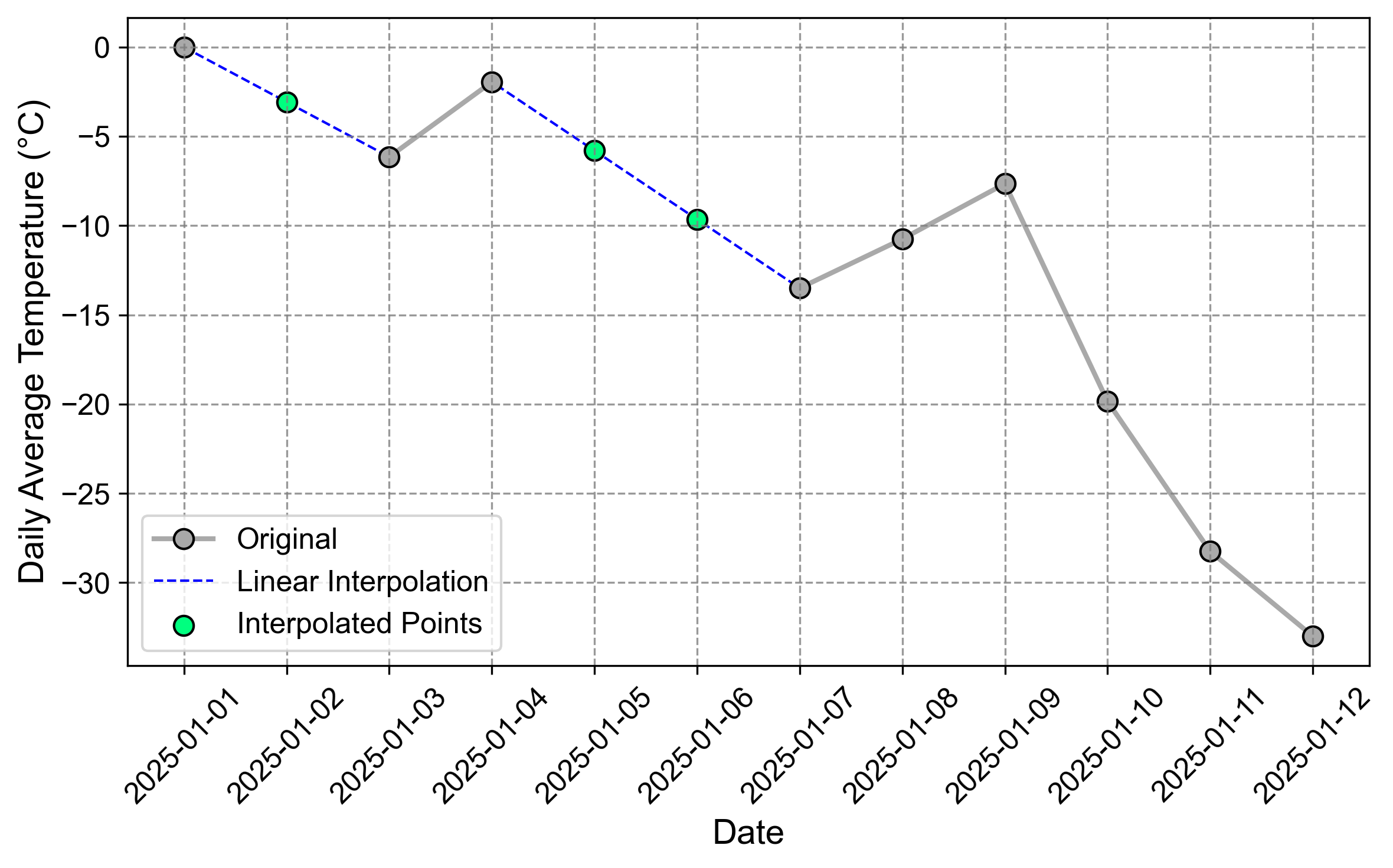
Fig. 2.11 Visualization of the time series after linear interpolation.

Fig. 2.11 illustrates how linear interpolation creates straight-line segments between known data points to estimate missing values. For example, between January 4th (-2.0°C) and January 7th (-13.5°C), two missing values are interpolated at January 5th (-5.8°C) and January 6th (-9.650°C), following a constant rate of decrease. Similarly, the missing value on January 2nd is interpolated between January 1st (0.0°C) and January 3rd (-6.150°C).

Advantages and Limitations of Linear Interpolation

Advantages:

1. Simplicity: Linear interpolation is easy to implement and computationally efficient, making it a practical choice for many time-series datasets.

2. Preserves Dataset Structure: Retains all rows in the dataset by imputing missing values instead of removing them, ensuring continuity in time-series data.

3. Smooth Transitions: Produces reasonable estimates for missing values by maintaining smooth transitions between observed data points.

4. Applicability: Particularly effective for datasets where trends are stable or changes between observations are gradual.

Limitations:

1. Assumption of Linearity:

   • Assumes that changes between consecutive observations are linear, which may not hold true for datasets with non-linear trends.

2. Underestimates Variability:

   • Can reduce variability in the dataset by smoothing fluctuations, potentially distorting the time-series dependence structure [Hollingdale et al., 2018, Raubitzek and Neubauer, 2021].

3. Ineffectiveness for Long Gaps:

   • May produce inaccurate estimates when gaps are large or irregularly spaced [Kandasamy et al., 2013].

4. Not Suitable for Non-linear Trends:

   • For datasets with complex patterns, advanced interpolation methods (e.g., spline interpolation or curve fitting) may provide better results [Raubitzek and Neubauer, 2021].

Linear interpolation is a simple yet effective method for filling gaps in time-series data when changes between observations are approximately linear and gaps are short or regularly spaced:

1. Use linear interpolation for datasets with stable trends or gradual changes over time.

2. For datasets with non-linear trends or long gaps, consider alternative methods such as spline interpolation or machine learning-based imputation techniques.

2.3.3.2. Polynomial Interpolation

Polynomial interpolation fits a polynomial function through known data points to estimate missing values. Unlike linear interpolation which creates straight lines between points, polynomial interpolation can capture more complex patterns in the data. The order of the polynomial determines its flexibility and complexity:

• A second-order (quadratic) polynomial has the form: \(P(t) = a_0 + a_1t + a_2t^2\) This can model simple curves with one bend, suitable for data with a single peak or valley.

• A third-order (cubic) polynomial has the form: \(P(t) = a_0 + a_1t + a_2t^2 + a_3t^3\) This allows for more complex curves with up to two bends, making it more flexible but potentially more prone to overfitting.

Higher-order polynomials can capture increasingly complex patterns but may introduce unwanted oscillations between data points, especially when dealing with gaps in the data.

For polynomial interpolation, instead of connecting points with straight lines as seen in the figure, we fit a polynomial through the known points. Here are implementations using both second and third-order polynomials:

Show code cell source

Hide code cell source

import pandas as pd

df = pd.read_csv('chapter02_data/generated_sample_time_series_avg_temp.csv', index_col=0)
df.index = pd.to_datetime(df.index)

# Apply second-order polynomial interpolation
poly2_interpolated = df.interpolate(method='polynomial', order=2)
print("\nSecond-order Polynomial Interpolation Results:")
display(poly2_interpolated)

# Apply third-order polynomial interpolation
poly3_interpolated = df.interpolate(method='polynomial', order=3)
print("\nThird-order Polynomial Interpolation Results:")
display(poly3_interpolated)

Second-order Polynomial Interpolation Results:

	TEMP
Date
2025-01-01	0.000000
2025-01-02	-6.054847
2025-01-03	-6.150000
2025-01-04	-1.950000
2025-01-05	-3.442099
2025-01-06	-10.624593
2025-01-07	-13.500000
2025-01-08	-10.750000
2025-01-09	-7.650000
2025-01-10	-19.850000
2025-01-11	-28.250000
2025-01-12	-33.000000

Third-order Polynomial Interpolation Results:

	TEMP
Date
2025-01-01	0.000000
2025-01-02	-8.984820
2025-01-03	-6.150000
2025-01-04	-1.950000
2025-01-05	-4.165076
2025-01-06	-9.878666
2025-01-07	-13.500000
2025-01-08	-10.750000
2025-01-09	-7.650000
2025-01-10	-19.850000
2025-01-11	-28.250000
2025-01-12	-33.000000

To better understand how different polynomial interpolation methods handle missing values in our temperature dataset, let’s examine their performance. Our dataset contains missing temperature values on January 2nd, 5th, and 6th, which each method approaches differently based on their underlying mathematical principles.

These estimates show how different interpolation methods handle the missing values:

For January 2nd:

• Linear interpolation: -3.075°C

• Second-order polynomial: -6.052°C

• Third-order polynomial: -8.899°C

For January 5th:

• Linear interpolation: -5.800°C

• Second-order polynomial: -3.393°C

• Third-order polynomial: -3.937°C

For January 6th:

• Linear interpolation: -9.650°C

• Second-order polynomial: -10.504°C

• Third-order polynomial: -9.508°C

The differences between these methods are substantial:

• Linear interpolation creates straight lines between known points, producing the most straightforward estimates

• Second-order polynomial captures a single parabolic curve, resulting in notably different values, particularly for January 2nd (-6.052°C vs -3.075°C from linear)

• Third-order polynomial allows for more complex curves, leading to the most extreme estimate for January 2nd (-8.899°C) while providing intermediate estimates for January 5th and 6th

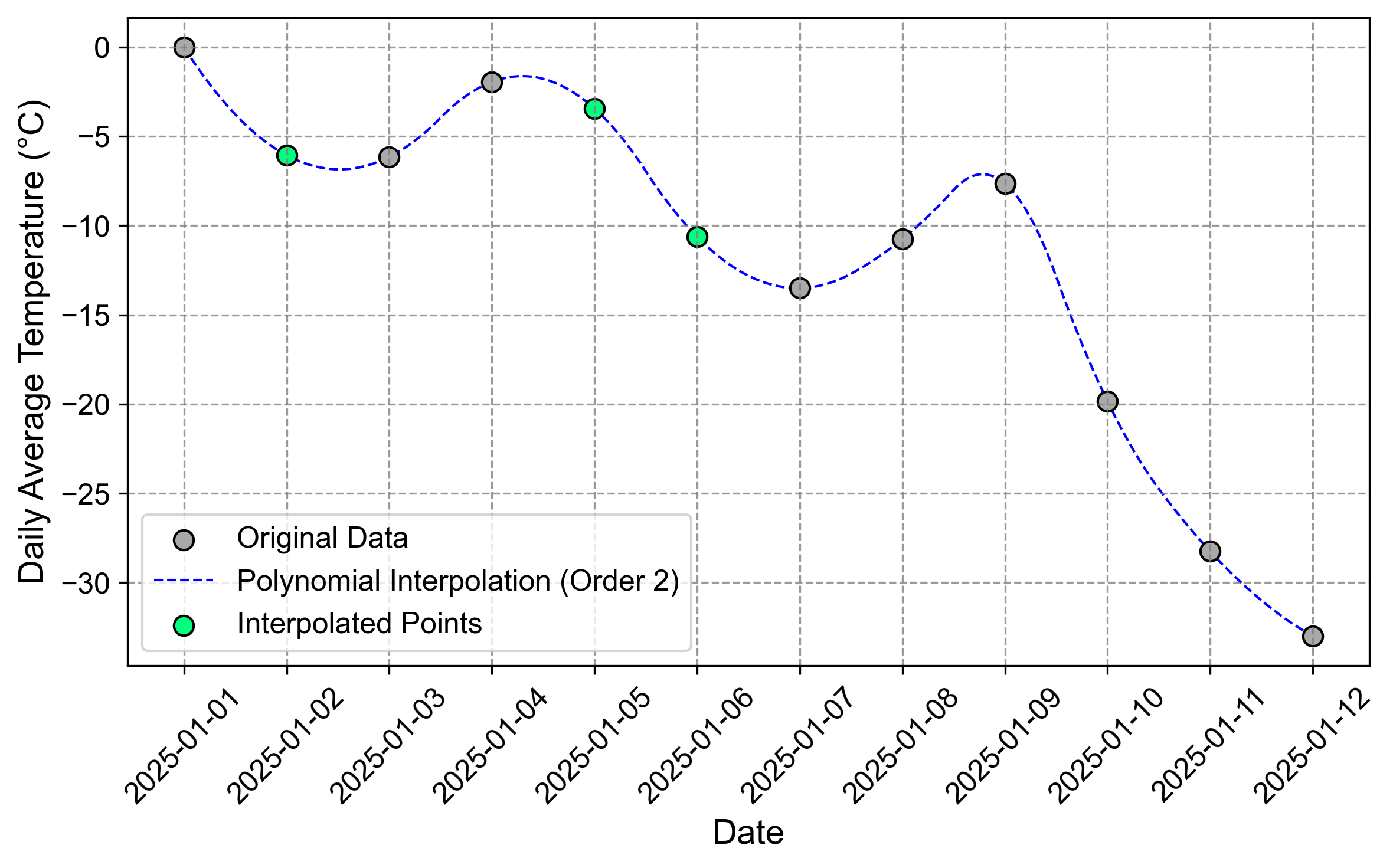
Fig. 2.12 Visualization of the time series after a quadratic (second-order) polynomial interpolation. The green curve shows how a simpler polynomial captures the general trend while potentially missing some local variations.

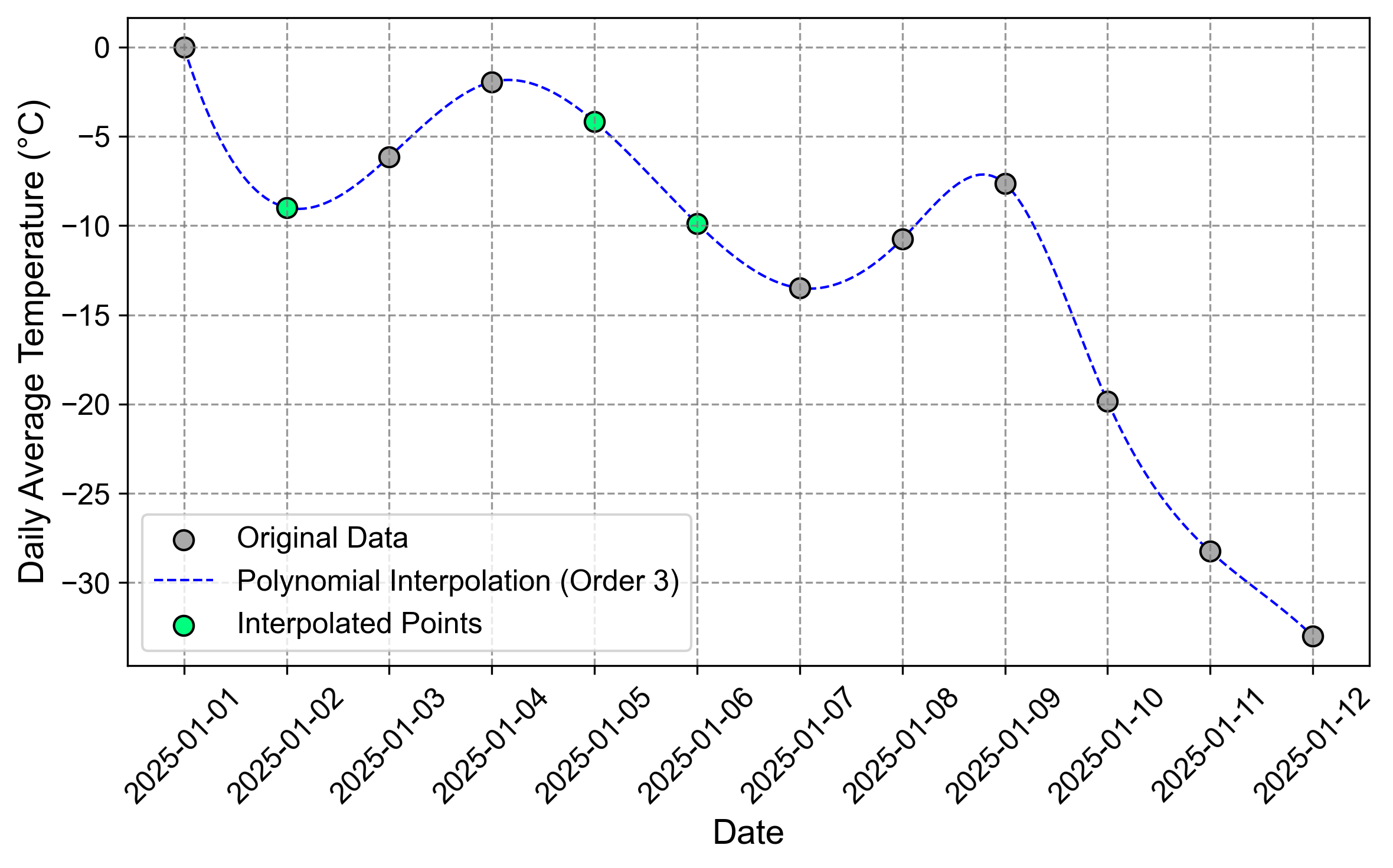
Fig. 2.13 Visualization of the time series after a cubic (third-order) polynomial interpolation. The blue curve demonstrates how a higher-order polynomial can capture more complex patterns in the temperature changes.

Fig. 2.12 and Fig. 2.13 illustrate the difference between second and third-order polynomial interpolation. The quadratic polynomial (order=2) provides a smoother fit with less flexibility, while the cubic polynomial (order=3) captures more local variations in the temperature pattern. The choice between these orders depends on the expected complexity of the underlying temperature changes and the risk of overfitting.

2.3.3.3. Spline Interpolation

Spline interpolation is a sophisticated technique used for enhancing low-resolution signals, data approximation, and interpolation. Unlike simpler methods, splines provide smooth transitions while avoiding oscillation problems common in high-degree polynomial interpolation [Bejancu, 2011, Bittencourt et al., 2017, Chen et al., 2023]. Let’s explore the main variants:

1. Linear spline: A linear spline is a type of spline function that is constructed piece-wise from linear functions creating two-point interpolating polynomials [Schmidt et al., 2019]. This means that the spline is composed of multiple linear segments, each defined by two points, and these segments are joined together at specific points, called knots [Schmidt et al., 2019].

   Linear splines are commonly used for interpolation and smoothing of data, particularly in cases where the data has a simple, linear relationship between the independent and dependent variables [Schmidt et al., 2019]. They are also used in various applications, such as data fitting, signal processing, and computer graphics [Schmidt et al., 2019].

   One of the advantages of linear splines is their simplicity and ease of implementation [Schmidt et al., 2019]. They can be easily constructed and evaluated, making them a popular choice for many applications. However, linear splines have some limitations, such as their inability to capture complex relationships between variables [Schmidt et al., 2019]. They are also sensitive to the choice of knots and can produce poor results if the knots are not carefully selected [Schmidt et al., 2019].

   Linear splines can be used in various applications, such as:

   • Data interpolation: Linear splines can be used to interpolate data between given points [Schmidt et al., 2019].

   • Signal processing: Linear splines can be used to smooth and filter signals [Schmidt et al., 2019].

   • Computer graphics: Linear splines can be used to create smooth curves and surfaces [Schmidt et al., 2019].

2. Cubic Spline: Cubic splines are defined as a set of cubic polynomials that connect given points, with matching first and second derivatives at the junctions between polynomials. This method is widely used in mathematics, engineering, computer graphics, and scientific computing due to its smoothness, flexibility, accuracy, ease of implementation, and numerical stability[Muzaffar et al., 2024].

   The interpolation process involves dividing the interval between adjacent points into equal subintervals and using the resulting intermediate points as control points to constrain the curve’s curvature. For example, in our temperature dataset, when interpolating between January 4th (-1.95°C) and January 7th (-13.5°C), the method creates a smooth curve that maintains continuity in both first and second derivatives.

   One key advantage of cubic splines is their ability to handle data with jump discontinuities by using separate cubic spline approximations on either side of the discontinuity [Muzaffar et al., 2024]. However, the method also has limitations. It assumes the existence of first and second-order derivatives at interpolated points, which may not always hold true [Bai et al., 2012]. Additionally, the resulting curve can be sensitive to the choice of control points, potentially affecting smoothness and accuracy [Bai et al., 2012].

   Applications of cubic splines extend beyond simple interpolation to include:

   • Robot path planning [Lian et al., 2020]

   • Drawing geographic maps

   • Approximating functions with jump discontinuities [Muzaffar et al., 2024]

   • Construction of quadratic splines for quantile estimation

3. Third-order spline: Third-order spline interpolation is a fast, efficient, and robust way to interpolate functions [Schiesser, 2017]. It is based on the principle of dividing the interpolation interval into small segments, with each segment specified by a third-degree polynomial [Schiesser, 2017]. The coefficients of the polynomial are selected in such a way that certain conditions are met, depending on the interpolation method [Schiesser, 2017]. Third-order splines can be used to represent functional dependencies in the form of sums of paired products of constant coefficients by the values of basis functions, providing the basis for significant parallelization of calculations [Schiesser, 2017].

   A third-order spline basis can effectively represent the shape of a deformable linear object (DLO). The spline basis is a function of a free coordinate u, which represents the position on the DLO. The spline basis is used to define the DLO’s dynamic model, which includes the total kinetic energy, external forces, and potential energy . The potential energy is generated due to the influence of gravity, stretching, torsion, and bending effects on the DLO.

   Third-order spline interpolation is used in various applications, including lane detection for intelligent vehicles [Cao et al., 2019]. An n-order B-spline curve is defined as a function of position vectors and basis functions [Cao et al., 2019]. A third-order B-spline curve is used to fit lane lines in complex road conditions, and the mathematical expression corresponding to the curve is given [Cao et al., 2019].

   Exponential splines are also used to find the numerical solution of third-order singularly perturbed boundary value problems [Wakjira and Duressa, 2020]. The exponential spline function is presented to solve the problem, and convergence analysis is briefly discussed [Wakjira and Duressa, 2020]. The method is shown to be sixth order convergence [Wakjira and Duressa, 2020]. The applicability of the method is validated by solving some model problems for different values of the perturbation parameter, and the numerical results are presented both in tables and graphs [Wakjira and Duressa, 2020].

4. PCHIP (Piecewise Cubic Hermite Interpolating Polynomial): PCHIP offers a shape-preserving alternative to cubic splines by maintaining monotonicity in the interpolated values. While sacrificing some smoothness, it better preserves local trends and avoids introducing artificial extrema in the data.

   Recent applications of spline interpolation include:

   • Sound field estimation using physics-informed neural networks [Shigemi et al., 2022]

   • Robot path planning with cubic spline interpolation [Lian et al., 2020]

   • Bearing fault diagnosis using B-spline-based deep learning [Li et al., 2024]

   While spline interpolation offers advantages in approximating complex functions and handling high-dimensional data, it’s important to consider its computational complexity and potential for oscillation near data points when choosing an interpolation method [Bejancu, 2011, Bittencourt et al., 2017, Chen et al., 2023].

5. B-Spline (Basis Spline): B-splines are sophisticated mathematical functions used to construct curves and surfaces through piecewise-defined polynomial curves, smoothly blended between control points. They are extensively used in computer-aided design (CAD), geometric modeling, and image processing due to their ability to create continuous and smooth curves that can be extended to higher dimensions [Rehemtulla et al., 2022].

   A key advantage of B-splines is their non-parametric nature, allowing them to model curves without restricting velocity or density profiles to specific shapes [Rehemtulla et al., 2022]. They can represent complex nonlinear mappings as combinations of piecewise polynomials, enhancing model expressiveness when handling continuous functions [Li et al., 2024]. This flexibility makes them particularly valuable for:

   • Creating reference trajectories in trajectory planning [Tao et al., 2024]

   • Modeling cusps or jumps at interfaces while maintaining differentiability elsewhere

   • Guiding autonomous systems through dynamic environments [Tong et al., 2024]

   B-splines excel in applications requiring precise curve modeling, from trajectory planning to density profile estimation in astrophysics[Rehemtulla et al., 2022]. Their ability to maintain smoothness while accommodating complex patterns makes them particularly suitable for handling real-world data with varying degrees of complexity.

   1. Akima spline: Akima spline is a type of cubic spline interpolation method that is widely used in various fields, including signal processing, image processing, and machine learning. It is a locally supported interpolation method, meaning that the value of the spline at a given point is determined by its neighborhood. This makes Akima spline more efficient and effective than other interpolation methods, such as cubic splines, which are global and can lead to unnatural wiggles in the resulting curve.

   One of the key advantages of Akima spline is its ability to balance the continuity of the interpolation function and calculation costs [Yang et al., 2023]. It uses a unique cubic polynomial to determine the spline curve between every pair of consecutive points, and the coefficients of the polynomials are determined by four constraints [Yang et al., 2023]. This ensures that the Akima spline function and its first derivatives are continuous, making it a popular choice for various applications.

   Akima spline has been used in various fields, including signal processing [Gupta and Cornish, 2024], image processing [Martínez Sánchez et al., 2019], and machine learning [Yang et al., 2023]. In signal processing, Akima spline is used to reconstruct signals from level-crossing samples. In image processing, it is used for fast ground filtering of airborne LiDAR data [Martínez Sánchez et al., 2019]. In machine learning, Akima spline is used for interpolation and extrapolation tasks, such as in Bayesian power spectral estimation [Gupta and Cornish, 2024] and quantum cluster theories [Maier et al., 2005].

   In addition to its applications, Akima spline has also been compared to other interpolation methods, such as cubic splines and Hermite interpolation polynomials[Yang et al., 2023]. The results show that Akima spline outperforms these methods in terms of accuracy and efficiency.

6. Thin Plate Spline: Thin plate splines are sophisticated interpolation methods designed for scattered data in high-dimensional spaces. They function as unique minimizers of the squared seminorm among all admissible functions taking prescribed values at given points. This method has gained prominence in computer-aided design, engineering, and remote sensing applications.

   Key advantages of thin plate splines include:

   • Ability to handle high-dimensional data

   • Invariance to rotations or reflections of coordinate axes [Kalogridis, 2023]

   • Computational efficiency with only one smoothing parameter [Kalogridis, 2023]

   The method has found particular success in remote sensing applications, where it generates reference surfaces for filtering algorithms [Cheng et al., 2019]. For example, in terrain analysis, thin plate splines can create reference surfaces that reflect terrain fluctuations, enabling the removal of nonground points through iterative processing [Cheng et al., 2019].

   Recent developments include low-rank thin plate splines (LR-TPS), which achieve comparable estimation accuracy to traditional thin plate splines but with significantly reduced computational time. These advances have made the method particularly valuable for dynamic function-on-scalars regression and other applications requiring efficient processing of complex, high-dimensional data.

Beyond the spline methods discussed above, several other variants exist. Smoothing splines incorporate a roughness penalty to balance fit and smoothness [Wang, 2011]. Tension splines allow control over the “tightness” of the curve through a tension parameter [Kvasov, 2000]. Cardinal splines offer local control over curve characteristics while maintaining continuity [Schoenberg, 1973]. Natural cubic splines enforce zero second derivatives at endpoints, making them useful for physical systems [Fahrmeir et al., 2013]. Catmull-Rom splines are particularly popular in computer graphics for their local control properties [Goldman, 2002]. Quasi-interpolating splines provide approximations that don’t necessarily pass through all data points but maintain important shape properties [Buhmann et al., 2022].

In the following sections, we will demonstrate the application of three commonly implemented spline methods - cubic spline, PCHIP, and Akima spline - using our synthetic daily average temperature dataset. These methods are available through scipy.interpolate and pandas, making them readily accessible for time series interpolation tasks. We’ll examine how each method handles the missing temperature values on January 2nd, 5th, and 6th, comparing their behavior and appropriateness for meteorological data.

Show code cell source

Hide code cell source

import pandas as pd

# Load the dataset
df = pd.read_csv('chapter02_data/generated_sample_time_series_avg_temp.csv', index_col=0)
df.index = pd.to_datetime(df.index)
spline_dict = {'First order spline (linear spline)': 'slinear',
               'Cubic spline': 'cubicspline',
               'Third order spline': 'cubic',
               'Piecewise Cubic Hermite Interpolating Polynomial': 'pchip',
               'Akima spline': 'akima',}

# Specify order for methods that require it
data = {}
for name, method in spline_dict.items():
    data[name] = df.interpolate(method=method)

df_comparison = pd.concat(data, axis=1)
df_comparison.columns = [name for name in spline_dict.keys()]

display(df_comparison)

	First order spline (linear spline)	Cubic spline	Third order spline	Piecewise Cubic Hermite Interpolating Polynomial	Akima spline
Date
2025-01-01	0.000	0.000000	0.000000	0.000000	0.000000
2025-01-02	-3.075	-8.984820	-8.984820	-5.056250	-4.847762
2025-01-03	-6.150	-6.150000	-6.150000	-6.150000	-6.150000
2025-01-04	-1.950	-1.950000	-1.950000	-1.950000	-1.950000
2025-01-05	-5.800	-4.165076	-4.165076	-4.944444	-5.503694
2025-01-06	-9.650	-9.878666	-9.878666	-10.505556	-11.610180
2025-01-07	-13.500	-13.500000	-13.500000	-13.500000	-13.500000
2025-01-08	-10.750	-10.750000	-10.750000	-10.750000	-10.750000
2025-01-09	-7.650	-7.650000	-7.650000	-7.650000	-7.650000
2025-01-10	-19.850	-19.850000	-19.850000	-19.850000	-19.850000
2025-01-11	-28.250	-28.250000	-28.250000	-28.250000	-28.250000
2025-01-12	-33.000	-33.000000	-33.000000	-33.000000	-33.000000

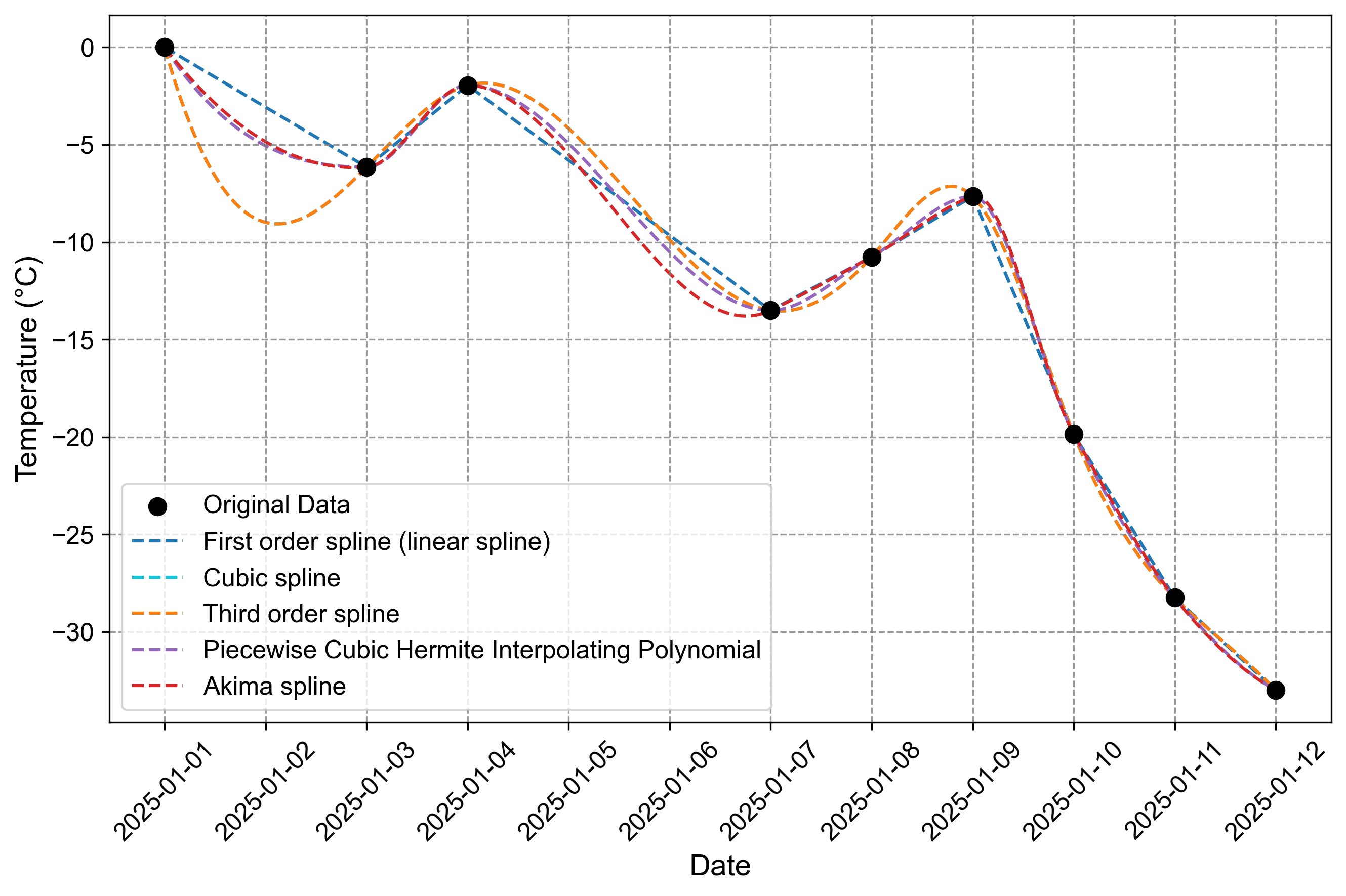
Fig. 2.14 Comparison of different spline interpolation methods for temperature data interpolation. The figure shows various interpolation techniques applied to temperature measurements from January 2025, with black dots representing actual measurements and different line styles showing interpolation results.

Fig. 2.14 shows a comparison of different spline interpolation methods used to fill missing temperature data points over a 12-day period in January 2025. The original temperature data (shown as black dots) contains several gaps, particularly on January 2nd, 5th, and 6th.

Original Data Pattern

• Starting at 0°C on January 1st

• Drops to -6.15°C by January 3rd

• Rises to -1.95°C on January 4th

• Falls again to -13.50°C by January 7th

• Shows a dramatic decline after January 9th, reaching -33°C by January 12th

Method Behaviors

Table 2.8 Comparison of Interpolation Methods for Temperature Data

Method	Key Characteristics	Interpolation Behavior
Linear Spline	Direct point-to-point connection	Most conservative, minimal oscillation
Cubic/Third Order	Higher-order polynomial fitting	Produces smooth curves with potential overshooting
PCHIP	Shape-preserving interpolation	Maintains data monotonicity with natural transitions
Akima	Robust to outliers	Balanced between smoothness and data fidelity

Notable Observations

• The cubic and third-order splines show identical behavior, producing the most extreme interpolation around January 2nd (-8.98°C)

• The linear spline provides the most conservative estimates, with straight-line connections between known points

• All methods converge closely for the steep temperature drop between January 9th and 12th

• The Akima and PCHIP methods generally provide more moderate interpolations compared to the cubic splines

The graph effectively demonstrates how different interpolation techniques can produce varying estimates for the same missing data points, particularly evident in the gaps between January 1-3 and January 4-7.

2.3.4. Advanced Techniques for Handling Missing Data

While we have covered several fundamental approaches to handling missing data, there are more sophisticated methods that leverage advanced statistical and machine learning techniques. These approaches often require a deeper understanding of machine learning concepts, which we will explore in later chapters after covering various ML models.

One category of advanced techniques includes machine learning-based imputation methods. Random Forest Imputation, for example, uses the Random Forest algorithm to predict missing values based on other features in the dataset. This method can capture complex relationships and handle both numerical and categorical data effectively. Similarly, K-Nearest Neighbors (KNN) Imputation uses the K most similar records to estimate missing values, which is particularly useful when there are strong correlations between features.

Model-based methods offer another sophisticated approach to handling missing data. The Expectation-Maximization (EM) algorithm is an iterative method that estimates parameters in models with incomplete data by maximizing the likelihood function. Maximum Likelihood Estimation (MLE) directly estimates parameters from incomplete data and is often used in structural equation modeling or advanced statistical analyses.

Deep learning approaches have also been applied to the problem of missing data. Autoencoders, a type of neural network, can learn patterns in data and predict missing values based on learned representations. Generative Adversarial Networks (GANs) can generate realistic values to fill in gaps in datasets, which is particularly useful for complex data types like images.

Multiple imputation techniques, such as Multiple Imputation by Chained Equations (MICE), create multiple plausible imputed datasets, analyze each separately, and then combine the results. This method accounts for the uncertainty in the imputation process, providing more robust estimates.

These advanced techniques often provide more accurate imputations, especially for complex datasets with non-random missing patterns. However, they typically require a solid understanding of statistical and machine learning concepts. As we progress through subsequent chapters and delve deeper into machine learning models, we will revisit some of these methods and explore their implementation in greater detail.