Automated ARIMA Models

4.7. Automated ARIMA Models#

4.7.1. Introduction#

Throughout this chapter, we have emphasized a systematic and disciplined approach to ARIMA modeling: testing for stationarity, carefully examining ACF and PACF plots, performing manual grid searches across candidate parameters, and comparing models using information criteria. This workflow offers distinct advantages—we understand the rationale behind each parameter selection, we can justify our choices to stakeholders, and we maintain complete control over the modeling process. However, this traditional approach is computationally expensive and labor-intensive, often requiring extensive visualization and iterative fitting across numerous parameter combinations.

Auto-ARIMA represents a fundamentally different philosophy. Instead of manually specifying candidate parameters, the algorithm automatically searches the \((p,d,q)(P,D,Q)_s\) parameter space to identify the model that optimizes a statistical criterion (typically AIC). This automation prioritizes speed and objectivity over interpretability, facilitating rapid model selection when domain knowledge is limited or when we must forecast hundreds of time series at scale.

4.7.2. The Stepwise Search Algorithm#

Auto-ARIMA employs a stepwise search strategy that mirrors manual analysis but operates with significantly greater computational efficiency. The process typically unfolds as follows:

Determine Differencing Orders: The algorithm applies unit root tests (such as ADF or KPSS) to identify the number of regular differences (\(d\)) and seasonal differences (\(D\)) required to achieve stationarity.
Initialize with Simple Models: The search begins with parsimonious parameter values (e.g., \(p=0, q=0, P=0, Q=0\)).
Explore Parameter Space: The algorithm incrementally perturbs parameters by \(\pm 1\), fitting new candidate models at each step.
Select Best Model: At each iteration, the model with the lowest AIC is retained as the current champion.
Terminate Search: The process concludes when parameter perturbations no longer yield a reduction in AIC.

Note

The algorithm does not perform an exhaustive search of every possible \((p,d,q,P,D,Q)_s\) combination, as this would require thousands of model fits even for moderate parameter bounds. Instead, stepwise pruning explores only locally promising parameter neighborhoods, reducing computation time from hours to seconds. This efficiency is the core advantage of the automated approach.

Advantages of Auto-ARIMA

Speed and Efficiency: Auto-ARIMA fits dozens of candidate models in seconds. In contrast, manual analysis—producing plots, interpreting correlations, and fitting grid search candidates—can easily consume hours for a single series. This speed is critical when forecasting high-volume portfolios in production environments.
Objectivity: The algorithm eliminates subjective judgment from ACF and PACF interpretation. There is no ambiguity about whether a specific lag is “significant enough” to warrant inclusion; the criterion is strictly whether it reduces the AIC. This objectivity ensures consistency and auditability in operational settings.
Enterprise Scalability: While manual analysis is feasible for a handful of series, it becomes impractical for forecasting 500 or 5,000 items. Auto-ARIMA handles batch processing efficiently, generating reasonable baseline models across large datasets with minimal human intervention.
Rapid Baseline Development: Auto-ARIMA quickly establishes whether a time series requires complex structures or if simple specifications suffice. This provides a valuable initial benchmark during the exploratory phase of a project.
Accessibility: By abstracting away the complexities of differencing logic and lag interpretation, Auto-ARIMA enables practitioners with limited time series expertise to generate robust models.

Limitations and Pitfalls

In-Sample Optimization Bias: Auto-ARIMA optimizes AIC, which is calculated on the training data. A model with the lowest AIC may not necessarily perform best on unseen future data—a classic manifestation of the bias-variance tradeoff.
Preference for Unnecessary Complexity: When AIC improvements are marginal, the algorithm may favor models with additional parameters. This can lead to overparameterized models that fit training noise rather than the underlying signal, degrading out-of-sample performance.
Loss of Interpretability: The algorithm operates as a “black box,” providing no causal explanation for its parameter selection. It may be difficult to explain to stakeholders why a specific AR term was included or why a seasonal difference was omitted.
Neglect of Domain Knowledge: The algorithm lacks context. It may select a statistically optimal model that produces forecasts contradicting physical or business realities—such as negative sales or impossible inventory levels.
Incomplete Residual Validation: Auto-ARIMA does not routinely verify that residuals exhibit white noise properties. A model selected for its low AIC may still suffer from autocorrelation, indicating specification inadequacy. Manual residual diagnostics remain essential.

Best Practice

We should treat Auto-ARIMA as a starting point and benchmark, not a final solution. It is imperative to validate selected models through rigorous residual diagnostics and out-of-sample forecast evaluation before deployment.

4.7.3. Example: Comparing Manual vs. Auto-ARIMA on Airline Passengers#

Let’s compare both approaches on the canonical Airline Passengers dataset (1949–1960). This dataset is considered the “Hello World” of seasonal time series forecasting and was the primary case study used by Box and Jenkins to demonstrate the power of seasonal ARIMA modeling.

4.7.3.1. The Manual Approach#

Through our previous analysis (or simply by following Box and Jenkins’ classic derivation), we identified the SARIMA(0,1,1)(0,1,1,12) specification as the gold standard for this data. The logic is elegant and transparent:

\(d=1\): Regular differencing removes the linear trend.
\(D=1\): Seasonal differencing at lag 12 removes the annual cycle.
\(\theta_1, \Theta_1\): Moving average terms model the remaining smooth autocorrelation structure.

4.7.3.2. The Automated Approach#

Now we run Auto-ARIMA on the same training data. We enable the stepwise search and allow the algorithm to determine the optimal differencing and parameter orders based on minimizing AIC.

                                     SARIMAX Results                                      
==========================================================================================
Dep. Variable:                                  y   No. Observations:                  122
Model:             SARIMAX(2, 0, 0)x(0, 1, 0, 12)   Log Likelihood                -408.015
Date:                            Fri, 02 Jan 2026   AIC                            824.031
Time:                                    20:12:44   BIC                            834.833
Sample:                                01-31-1949   HQIC                           828.412
                                     - 02-28-1959                                         
Covariance Type:                              opg                                         
==============================================================================
                 coef    std err          z      P>|z|      [0.025      0.975]
------------------------------------------------------------------------------
intercept      4.9719      1.964      2.531      0.011       1.122       8.822
ar.L1          0.6745      0.099      6.826      0.000       0.481       0.868
ar.L2          0.1406      0.097      1.445      0.148      -0.050       0.331
sigma2        96.6711     11.946      8.093      0.000      73.258     120.084
===================================================================================
Ljung-Box (L1) (Q):                   0.00   Jarque-Bera (JB):                 1.36
Prob(Q):                              0.96   Prob(JB):                         0.51
Heteroskedasticity (H):               1.48   Skew:                            -0.02
Prob(H) (two-sided):                  0.24   Kurtosis:                         3.54
===================================================================================

Warnings:
[1] Covariance matrix calculated using the outer product of gradients (complex-step).

4.7.3.3. Accuracy metrics#

Table 4.9 presents a side-by-side comparison of the Manual and Auto-ARIMA models across key performance dimensions.

Table 4.9 Quantitative Comparison#
	Manual SARIMA	Auto-ARIMA
AIC	723.84	824.03
BIC	731.51	834.83
Parameters	3	4
Training RMSE	16.06	32.94
Training MAPE (%)	5.04	10.64
Test RMSE	45.29	39.87
Test MAPE (%)	8.80	7.69

In-Sample Superiority (Manual Model): The Manual SARIMA(0,1,1)(0,1,1,12) clearly outperforms Auto-ARIMA on the training data. Its AIC (723.84) is over 100 points lower than the Auto-ARIMA model (824.03), and its training RMSE (16.06) is roughly half that of the automated model (32.94). This confirms that the manual specification—which explicitly removes the stochastic trend and seasonal cycle via differencing—captures the historical data structure far more efficiently.
Structural Differences (The “Stiffness” Factor): The Auto-ARIMA output reveals why the models behave differently. The automated selection is SARIMA(2,0,0)(0,1,0,12) with intercept.
- Intercept: The coefficient is 4.97 (\(p=0.011\)), enforcing a deterministic upward drift.
- AR Terms: The first AR lag is 0.67 (\(p<0.001\)), creating strong persistence around that deterministic trend.
This structure creates a “stiff” model that rigidly projects the historical slope forward. In contrast, the manual model’s differencing (\(d=1\)) allows the trend to evolve stochastically, adapting to shocks rather than forcing a fixed trajectory.
Out-of-Sample Performance (Mixed Bag): On the test set, the Auto-ARIMA model achieves a lower RMSE (39.87 vs 45.29) and MAPE (7.69% vs 8.80%). This suggests that for this specific short-term horizon, the rigid deterministic trend of the Auto-ARIMA model happened to extrapolate the trajectory slightly better than the stochastic trend of the manual model.
Parsimony vs. Complexity: The manual model achieves its results with fewer parameters (3 vs. 4). The significant gap in BIC (731.51 vs. 834.83) heavily penalizes the Auto-ARIMA model for its inefficiency.

While Auto-ARIMA provides a marginally better forecast on the test set, the Manual SARIMA model remains preferable for robust operational use. It offers a theoretically sound representation of the data generating process (stochastic trend/seasonality), fits the historical record much better, and avoids the risk of a deterministic trend that could dangerously diverge over longer horizons. The Auto-ARIMA model is arguably “right for the wrong reasons”—it fits a rigid curve that happened to align with the test data, but lacks the adaptive capacity of the properly differenced manual model.

4.7.4. Forecast Performance Evaluation#

Having established the two competing models—the manually identified SARIMA(0,1,1)(0,1,1,12) and Auto-ARIMA’s selected SARIMA(2,0,0)(0,1,0,12) with intercept—we now turn to the critical question: how well do they forecast on unseen data? While in-sample fit statistics (AIC, BIC) provide useful information about model parsimony and data fit during training, the ultimate test of a time series model lies in its ability to accurately predict values it has never seen before. This out-of-sample forecast evaluation reveals which model truly generalizes better.

4.7.4.1. Generating Forecasts#

We generate forecasts for the held-out test set, which covers the final 24 months of the dataset (1959–1960). The manual model produces forecasts using statsmodels’ get_forecast() method, which returns both point predictions and 95% confidence intervals. Similarly, Auto-ARIMA’s predict() method provides comparable probabilistic outputs, allowing us to evaluate not just the accuracy of the point forecasts but also the reliability of the uncertainty bounds.

We visualize the trajectories of both models against the actual passenger counts for 1959–1960 to assess which specification captures the final evolution of the trend and seasonal cycle more accurately.

4.7.4.2. Visualizing Forecast Performance#

Fig. 4.29 provides a direct visual comparison of how each model performs on the test set (1959–1960). The plots display the training data in green, the actual test observations in blue, and the model forecasts in red.

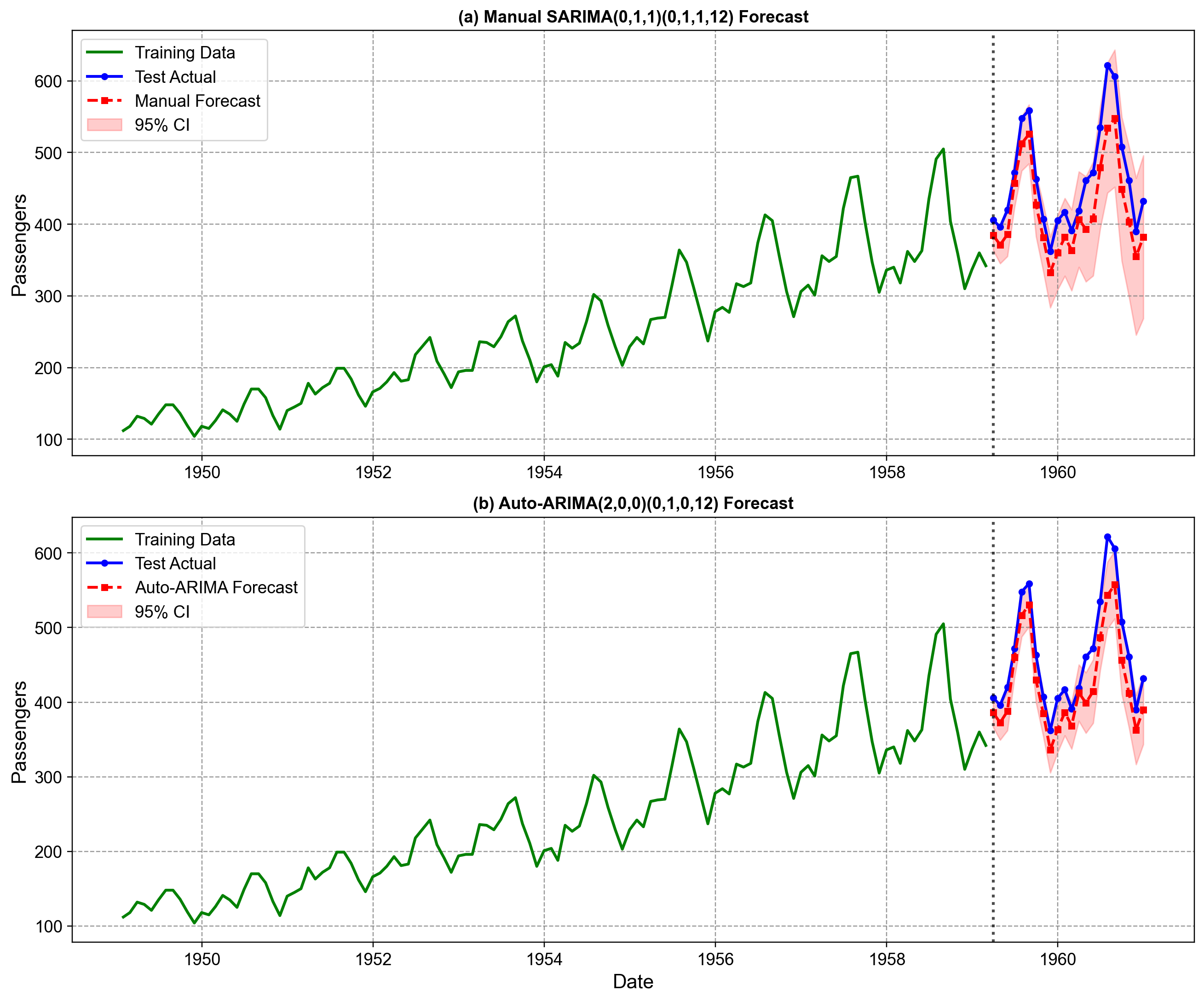
../_images/forecast_comparison.png — Fig. 4.29 **Comparison of manual SARIMA vs. Auto-ARIMA forecasts on Airline Passengers.** The top panel (a) displays forecasts from the manually identified **SARIMA(0,1,1)(0,1,1,12)**, while the bottom panel (b) shows the **Auto-ARIMA SARIMA(2,0,0)(0,1,0,12)** selection. Both models successfully capture the pronounced annual seasonality, tracking the timing of peaks (summer travel) and troughs (winter) throughout the 24-month horizon. The manual model’s confidence intervals (shaded red) widen noticeably more than the Auto-ARIMA intervals as the horizon extends. This reflects the theoretical difference in their structures: the manual model’s stochastic trend (\(d=1\)) accumulates uncertainty over time, whereas the Auto-ARIMA model’s deterministic trend (intercept + AR) implies a more rigid future path with tighter, though potentially overconfident, bounds [image:32].#

Trajectory Tracking: Both models capture the general upward trend and the seasonal oscillation reasonably well. Neither model exhibits a massive systematic failure (e.g., predicting a flat line or missing the seasonal peaks entirely).
Uncertainty Estimation: A key difference lies in the confidence intervals. The manual model (panel a) produces wider confidence bands that expand as we forecast further into the future. This is a desirable property, reflecting the genuine uncertainty of extrapolating a stochastic trend. In contrast, the Auto-ARIMA model (panel b) produces noticeably narrower bands. While this might look “more precise,” it is arguably “overconfident”—it assumes the future trend will follow the fixed intercept slope rather than acknowledging that the trend itself could drift.
Peak Accuracy: Visually, the Auto-ARIMA model (bottom) seems to hit the peak values slightly better than the manual model in the second year (1960). This visual intuition aligns with the lower RMSE we observed in the quantitative table (39.87 vs 45.29).

While the eye can discern these broad patterns, determining which model is truly superior requires the rigorous quantitative comparison we performed earlier. The visual evidence confirms that both are plausible models, but they represent fundamentally different beliefs about how the future unfolds (stochastic vs. deterministic).

4.7.4.3. Forecast Error Visualization#

To better understand where and why forecast errors occur, we visualize the residuals (forecast errors) across the test period. Fig. 4.30 plots these errors for both models on the same axis.

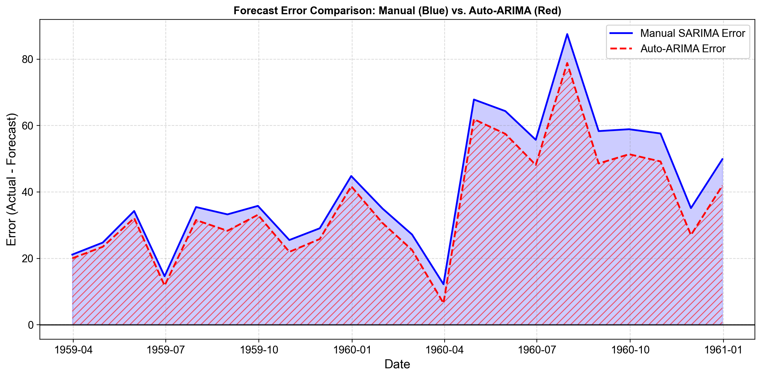
../_images/error_comparison.png — Fig. 4.30 **Forecast error comparison for Manual SARIMA (Blue) vs. Auto-ARIMA (Red) on Airline Passengers test data.** The blue solid line tracks the errors of the manual model, while the red dashed line tracks the Auto-ARIMA errors. Both models exhibit positive errors (under-forecasting) throughout the entire test period, with the magnitude peaking significantly during the summer months (July/August). This synchronized pattern reveals that both models struggle to capture the accelerating amplitude of the seasonal peaks in the final years of the dataset [image:35].#

Systematic Under-Forecasting: Unlike the “balanced” errors we typically hope for, both models consistently show positive errors (Actual > Forecast). The traces hover almost entirely above the zero line. This indicates that the trend in passenger growth during 1959-1960 accelerated faster than either the stochastic trend (Manual) or the deterministic trend (Auto-ARIMA) could project based on the training data.
Seasonal Amplitude Mismatch: The errors are not constant; they spike dramatically during the summer peaks (reaching nearly +90 for the Manual model and +80 for Auto-ARIMA). This suggests that the multiplicative seasonality is intensifying. While we log-transformed the data (or relied on the model to handle it), the extreme growth in peak travel is still being underestimated by both specifications.
Magnitude Comparison: The Auto-ARIMA errors (red dashed line) generally stay closer to the zero line than the manual model’s errors (blue solid line), particularly during the extreme summer peaks. This visually confirms the lower RMSE (39.87 vs 45.29) we observed earlier. The “stiffer” Auto-ARIMA model happened to catch the high amplitude of the 1960 summer peak slightly better than the stochastic manual model.

The visual similarity between the two error traces reinforces that the models are structurally distinct but functionally related. They succeed and fail in the same months, driven by the same underlying irregularities in the passenger data, with Auto-ARIMA holding a slight edge in amplitude accuracy for this specific test window.

4.7.4.4. Error Distribution Analysis#

Understanding the distribution of forecast errors provides deeper insight into model performance than summary metrics alone. Fig. 4.31 displays the histograms of forecast errors for both models on the test set.

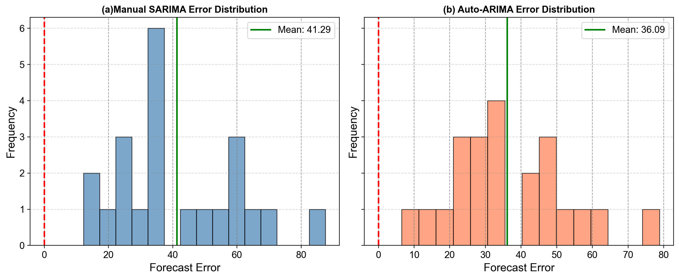
../_images/error_distributions.png — Fig. 4.31 **Distribution of forecast errors for Airline Passengers (1959–1960).** The left panel (a) displays manual SARIMA errors, while the right panel (b) shows Auto-ARIMA errors. The red dashed vertical line marks zero (perfect forecast), while the green solid line indicates the actual mean error. Unlike the Milk example, these distributions are **not** centered at zero. Both models show a significant positive bias (Mean Error > 36), indicating systematic under-forecasting. The distributions are somewhat multi-modal, reflecting the seasonal nature of the errors (large errors in peak months, smaller errors in off-peak months). Auto-ARIMA achieves a slightly lower mean error (36.09 vs 41.29) and lower standard deviation (17.34 vs 19.05), confirming its marginal advantage on this specific test window [image:36].#

Systematic Bias (Under-Forecasting): Both models exhibit a strong positive mean error: +41.29 for Manual SARIMA and +36.09 for Auto-ARIMA. This is a critical finding. It indicates that on average, the actual passenger counts were 36–41 passengers higher than predicted. This systematic under-prediction suggests that the trend in the final two years accelerated beyond what either model projected from the 1949–1958 training data.
Variability: The standard deviation of errors is slightly lower for Auto-ARIMA (17.34) compared to the Manual model (19.05). This aligns with the “stiffer” nature of the Auto-ARIMA specification—its deterministic trend happened to align better with the accelerated growth, leading to slightly tighter error clustering.
Skewness: Both distributions show positive skewness (~0.61–0.62). This “right tail” corresponds to the summer months, where the under-forecasting was most severe (errors reaching +80 or +90). The models struggle most with the extreme peaks.

4.7.5. When Should You Use Auto-ARIMA?#

The comparison between manual and automated selection reveals that the “best” approach depends heavily on your constraints: scale, stakes, and the need for explainability.

Appropriate Scenarios for Auto-ARIMA

Large-Scale Forecasting: If you must forecast 5,000 SKUs weekly, manual analysis is impossible. Auto-ARIMA allows you to trade a small amount of accuracy/explainability for the ability to scale.
Exploratory Baselines: Use Auto-ARIMA as a “sniff test” to quickly establish a performance floor. If your manual model cannot beat the automated baseline, you likely missed a signal in the ACF/PACF plots.
Low-Stakes/High-Volume: For routine operational metrics where individual errors have low cost, the speed of automation outweighs the benefits of deep inspection.

When Manual Analysis is Essential

High-Stakes Decision Making: When forecasts drive multi-million dollar inventory or staffing decisions, you must be able to explain why the model predicts a downturn. “The algorithm said so” is rarely a sufficient defense to stakeholders.
Long-Term Strategic Planning: As seen in our example, Auto-ARIMA can lock onto rigid deterministic trends that may diverge dangerously over long horizons. Manual analysis (\(d=1\)) ensures the model acknowledges structural uncertainty.
Structural Breaks & Anomalies: Automated tools blindly fit data. A human analyst can recognize that a dip in 2020 was due to a pandemic, not a permanent seasonal shift, and adjust the model accordingly.

4.7.6. Practical Workflow Recommendation#

The most robust approach is a hybrid workflow that leverages automation for efficiency while preserving human judgment for validity.

Run Auto-ARIMA First: Use it to get a quick read on the data complexity and establish a performance benchmark (AIC/RMSE).
Conduct Manual Diagnostics: Plot the ACF/PACF yourself. Does the automated model’s logic match the visual evidence? (e.g., Did it pick AR terms when you see clear seasonal spikes?)
Compete the Models: Fit both the automated suggestion and your manually derived specification.
Validate Out-of-Sample: Don’t rely on AIC alone. As we saw, a model with higher AIC (Auto-ARIMA) can sometimes forecast better in the short term, but you must assess if that performance is robust or lucky.
Check the Residuals: Ensure the final champion—regardless of how it was selected—produces white noise residuals.