Robust STL

3.4. Robust STL#

Robust STL extends the standard Seasonal-Trend decomposition using LOESS (STL) algorithm by incorporating an iterative reweighting process that automatically identifies and downweights outliers—extreme values that do not represent the time series’ underlying trend or seasonal structure. By progressively reducing the influence of observations with large residuals, Robust STL produces decomposition results that are far more resistant to distortion from anomalous data points [Wen et al., 2019].

3.4.1. The Vulnerability of Standard STL#

Standard STL relies on weighted least squares within its LOESS (Locally Estimated Scatterplot Smoothing) smoothers. While LOESS’s local weighting provides some natural robustness to minor deviations, the standard algorithm assumes all observations are approximately equally reliable. When severe outliers are present—whether from measurement errors, recording anomalies, or genuine but temporary extreme events—standard STL encounters several critical problems [Wen et al., 2019, Wen et al., 2020]:

Trend Distortion: Outliers exert undue influence on the fitted trend curve, creating spurious local bumps or dips that misrepresent the underlying long-term trajectory.
Seasonal Contamination: Outlier effects propagate through the LOESS smoothing of seasonal subseries, distorting the extracted seasonal patterns and producing irregular amplitudes during affected periods.
Residual Bleeding: Large residuals at outlier locations spread their influence to neighboring observations through the LOESS bandwidth, causing elevated residual variance beyond the immediate outlier time points.
Inflated Variance: Overall residual variance increases substantially, indicating that the decomposition has failed to cleanly separate systematic components from noise.

These pathologies are particularly problematic in real-world applications where data quality varies or where rare extreme events (e.g., financial crises, natural disasters, equipment failures) create temporary but severe deviations.

3.4.2. The Robust STL Solution: Iterative Reweighting#

Robust STL addresses these vulnerabilities through iterative reweighting based on residual magnitudes. The algorithm operates through two nested loops that progressively identify and downweight outliers:

3.4.2.1. Inner Loop (Standard STL Iteration)#

The inner loop executes the core STL decomposition using the current robustness weights, producing preliminary estimates of the trend ($T_t$), seasonal ($S_t$), and residual ($R_t$) components:

Detrending: Remove the previous trend estimate and apply seasonal LOESS to subseries
Low-pass filtering: Smooth the cycle-subseries component to obtain $S_t$
Deseasonalizing: Remove seasonal component and apply trend LOESS to obtain $T_t$
Residual computation: Calculate $R_t = y_t - T_t - S_t$

3.4.2.2. Outer Loop (Robust Reweighting)#

The outer loop, typically repeated 5–15 times until convergence, refines the observation weights:

After each inner loop, compute robustness weights $w_t$ based on standardized residuals $R_t$
Apply these updated weights to all LOESS fits in the next inner loop iteration
Continue iteratively until weights stabilize or maximum iterations are reached

The Key Result: Observations with large residuals (outliers) receive weights near zero ($w_t \approx 0$), effectively excluding them from trend and seasonal estimation without removing them from the dataset. Normal observations maintain full weight ($w_t \approx 1$), ensuring they drive the decomposition.

3.4.3. Mathematical Framework: Bisquare Weights#

The critical mechanism for robust downweighting is the bisquare (biweight) robustness function. This function calculates the weight $w_t$ after each inner loop using the following formula:

(3.13)#\[\begin{equation} w_t = \begin{cases} \left(1 - u_t^2\right)^2 & \text{if } |u_t| \leq 1 \\ 0 & \text{if } |u_t| > 1 \end{cases} \end{equation}\]

The calculation depends on the standardized residual ($u_t$):

(3.14)#\[\begin{equation} u_t = \frac{R_t}{c \cdot \text{MAD}(R)} \end{equation}\]

Here, $\text{MAD}(R)$ is the median absolute deviation ($\text{median}(|R_t - \text{median}(R)|)$). The MAD is a robust measure of scale that is highly resistant to outliers. The tuning constant, $c=6$, determines the threshold at which an observation receives a zero weight.

3.4.3.1. Understanding the Bisquare Function#

Table Table 3.6 illustrates the effect of the bisquare (biweight) robustness function on the weight assigned to an observation based on its standardized residual ($u_t$). This function is key to the robustness of the Robust STL method, providing a smooth and sophisticated way to downweight outliers compared to simple hard thresholding.

Table 3.6 Bisquare Weight Properties#
Residual Size	$u_t$ Value	Weight $w_t$	Interpretation
Normal (Small)	$u_t = 0$	$w_t = 1.00$	Full Influence (No downweighting)
Moderate	$u_t = 0.5$	$w_t = 0.56$	Reduced Influence (Partial downweighting)
Outlier Threshold	$u_t = 1.0$	$w_t = 0.00$	Zero Weight (Completely ignored)
Extreme (Outlier)	$u_t > 1.0$	$w_t = 0.00$	Completely Excluded

The table reveals several key features of the bisquare function. First, normal observations ($u_t = 0$) retain full weight, ensuring that well-behaved data points drive the decomposition. Second, moderate deviations ($u_t = 0.5$) receive substantial but not complete downweighting—this partial weight of 0.56 prevents these observations from exerting undue influence while still incorporating information from natural variability. Third, the sharp cutoff at $u_t = 1.0$ establishes a clear boundary: any observation whose standardized residual exceeds this threshold (corresponding to roughly 6 median absolute deviations) is completely excluded, preventing contamination of the extracted components.

3.4.3.2. How the Weighting Mechanism Works#

Normal Observations ($u_t = 0$): When a residual ($R_t$) is small (close to zero), the standardized residual $u_t$ is also zero. Plugging $u_t=0$ into the bisquare formula gives $w_t = (1 - 0^2)^2 = 1.00$. This ensures that observations that fit well with the current trend and seasonal estimates retain full influence in the subsequent LOESS fitting steps.
Moderate Deviations ($u_t = 0.5$): Observations with residuals that are moderately large, such that the standardized residual is $u_t = 0.5$, receive a partial weight of $w_t = (1 - 0.5^2)^2 = (1 - 0.25)^2 = 0.56$. This mechanism implements reduced influence, preventing these deviations from strongly pulling the fitted curves but still allowing them to contribute somewhat to the estimation.
The Outlier Threshold ($u_t = 1.0$): The value $u_t = 1.0$ acts as a definitive outlier threshold. At this point, the weight is $w_t = (1 - 1.0^2)^2 = 0.00$. Any observation whose standardized residual reaches or exceeds this value is effectively assigned a zero weight and is completely ignored in the calculation of the LOESS fits for the trend and seasonal components.
Extreme Outliers ($u_t > 1.0$): Any observation that is considered an extreme outlier (where $u_t$ exceeds 1.0) is also assigned a zero weight ($w_t = 0$). This means these points are completely excluded from the estimation, preventing them from contaminating the decomposition.

Algorithm 3.1 (Robust STL Algorithm)

Input Time series $y_t$, seasonal period $m$, window lengths (for LOESS fits)

Output The decomposed components: $T_t$ (trend), $S_t$ (seasonal), $R_t$ (residuals), and $w_t$ (robustness weights)

Initialize: Set the robustness weights $w_t \leftarrow 1$ for all time points $t$ (uniform initial weights).
Outer Loop (Robust Reweighting): FOR $outer\_loop = 1$ TO $n_{outer}$ (typically 5–15 iterations):
- a. Inner Loop (Standard STL Iteration): FOR $inner\_loop = 1$ TO $n_{inner}$:
  - i. Detrend: Calculate the detrended series $d_t \leftarrow y_t - T_t^{(k-1)}$.
  - ii. Weighted Seasonal LOESS: FOR each month (or season) $j = 1$ to $m$:
    - Fit LOESS to the seasonal subseries $d_j, d_{j+m}, d_{j+2m}, \dots$ using the current robustness weights $w_t$.
    - This yields the cyclic component $C_t^{(k)}$.
  - iii. Seasonal Component: Apply a weighted low-pass filter to $C_t^{(k)}$: $S_t^{(k)} \leftarrow \text{LowPass}(C_t^{(k)})$.
  - iv. Deseasonalize: Calculate the deseasonalized series $ds_t \leftarrow y_t - S_t^{(k)}$.
  - v. Weighted Trend LOESS: Fit LOESS to $ds_t$ using weights $w_t$: $T_t^{(k)} \leftarrow \text{LOESS}(ds_t)$.
  - vi. Residuals: Calculate the new residuals $R_t^{(k)} \leftarrow y_t - T_t^{(k)} - S_t^{(k)}$.
- b. Compute Robustness Weights: Calculate the new weights $w_t^{(new)}$ based on the residuals $R_t^{(k)}$:
  - i. $\text{median}_R \leftarrow \text{median}(R_t^{(k)})$
  - ii. $\text{MAD} \leftarrow \text{median}(|R_t^{(k)} - \text{median}_R|)$
  - iii. Calculate the standardized residual $u_t \leftarrow |R_t^{(k)}| / (c \times \text{MAD})$, where $c = 6$.
  - iv. Apply Bisquare Function: FOR $t = 1$ TO $N$:
    - IF $u_t \leq 1$: $w_t^{(new)} \leftarrow (1 - u_t^2)^2$
    - ELSE: $w_t^{(new)} \leftarrow 0$
  - v. Update weights: $w_t \leftarrow w_t^{(new)}$.
RETURN $T_t, S_t, R_t, w_t$

3.4.4. Example 1: Synthetic Outliers in CO₂ Data#

When learning about robust time series methods, it’s helpful to start with a controlled example where we know exactly what the problems are. To demonstrate how Robust STL handles outliers, we’ll use the monthly atmospheric CO₂ concentration data you’ve seen earlier in this course (familiar from {numref_stk_}), but with a twist: we’ll deliberately introduce some problematic data points.

In real-world time series analysis, outliers are unfortunately common. They can come from measurement errors, instrument malfunctions, data recording mistakes, or other anomalies. By artificially adding outliers to clean data, we can clearly see how different decomposition methods handle these problems. This controlled experiment lets us understand exactly what’s happening before tackling messier real-world data.

Introduced 8 outliers
Outlier dates: ['1967-05', '1971-02', '1978-03', '1981-07', '1985-04', '1965-09', '1974-11', '1982-05']

We’ve taken the clean CO₂ series and introduced 8 synthetic outliers at specific time points. Five are large positive spikes (adding 15-25 ppm to simulate sudden measurement jumps), and three are large negative drops (subtracting 10-18 ppm to simulate instrument drift). These outliers appear at dates like May 1967, February 1971, and so on—scattered throughout the series to show different scenarios.

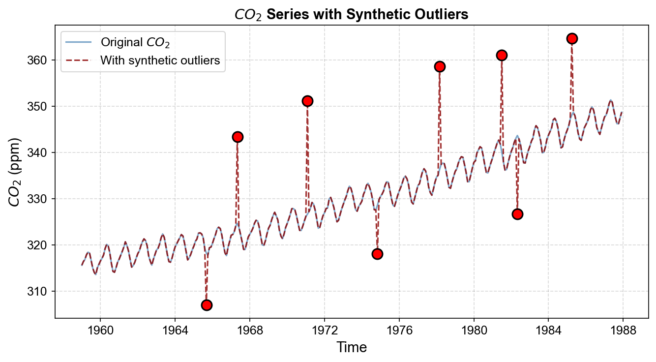
../_images/co2_with_outliers.png — Fig. 3.18 Monthly atmospheric CO₂ concentration with 8 synthetic outliers introduced (red circles). These outliers simulate measurement errors, instrument malfunctions, or data recording anomalies that can occur in real observational datasets.#

As you can see in Fig. 3.18, the red circles mark our intentionally corrupted observations. The original smooth trend is now interrupted by these extreme values. This is exactly the kind of messy data that challenges standard decomposition methods.

3.4.4.1. Standard vs. Robust STL: CO₂ Example#

Now comes the crucial question: how do these two methods handle the contaminated data? We ran both algorithms on the same corrupted CO₂ series using identical parameters (12-month seasonal period, seasonal window of 13).

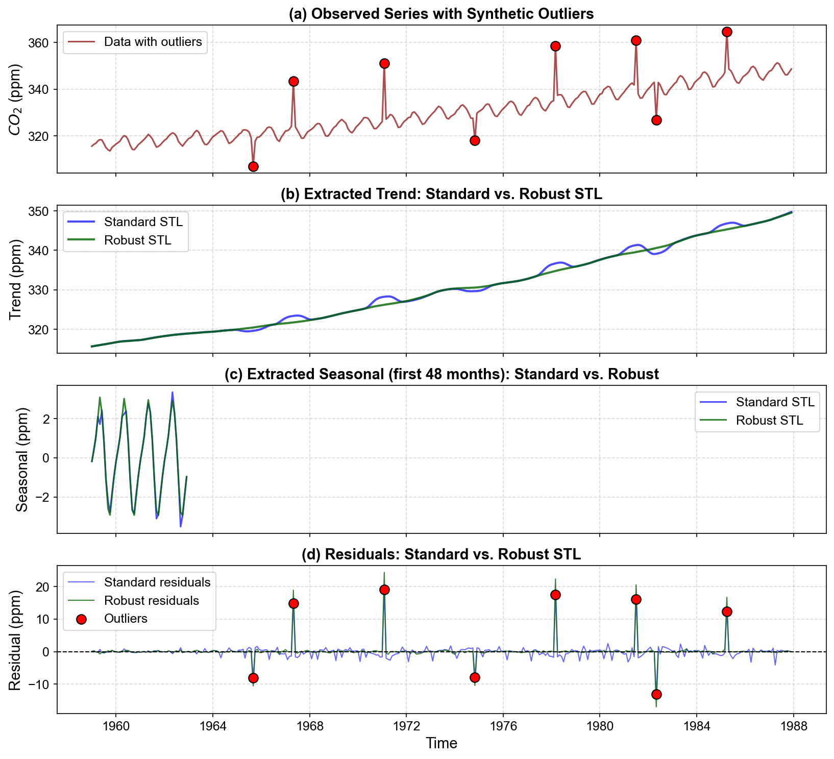
../_images/co2_standard_vs_robust.png — Fig. 3.19 Comparison of standard (non-robust) versus robust STL decomposition on CO₂ data with synthetic outliers. **(a)** Observed series with 8 outliers (red circles). **(b)** Trend components: Standard STL exhibits visible distortions (local bumps/dips) near outlier locations, while robust STL maintains smooth trend continuity. **(c)** Seasonal patterns (first 48 months): Standard STL shows irregular seasonal shapes where outliers appear; robust STL preserves consistent seasonal structure. **(d)** Residuals: Standard STL produces elevated residuals not only at outlier locations but also in neighboring points (contamination effect). Robust STL isolates large residuals exclusively at outlier positions.#

When examining the decomposition results across the four panels, pay attention to several key differences:

Panel (a) - The Contaminated Data: This shows our starting point—the CO₂ series with 8 outliers marked in red. Both algorithms receive the exact same input.
Panel (b) - Trend Extraction: Here’s where the differences become obvious. The standard STL trend (blue line) shows visible bumps and dips near each outlier location. These distortions mean the algorithm is being “fooled” by the outliers—it’s trying to fit them as part of the true underlying trend. In contrast, the robust STL trend (green line) maintains much smoother continuity, treating the outliers as temporary anomalies rather than real features of the trend.
Panel (c) - Seasonal Patterns: Looking at just the first 48 months for clarity, we can see that standard STL produces irregular seasonal shapes that vary depending on whether outliers are nearby. Robust STL preserves consistent seasonal patterns throughout the series, indicating it hasn’t let the outliers contaminate the seasonal component.
Panel (d) - Residuals: This panel reveals a subtle but important point. Standard STL not only has large residuals at the outlier locations (which we’d expect) but also shows elevated residuals in neighboring time points—this is the “residual bleeding” problem where outlier effects spread through the LOESS smoothing window. Robust STL cleanly isolates the large residuals to just the outlier positions themselves.

3.4.4.2. Robustness Weights Visualization#

So how does Robust STL achieve this superior performance? The answer lies in the robustness weights that the algorithm automatically calculates.

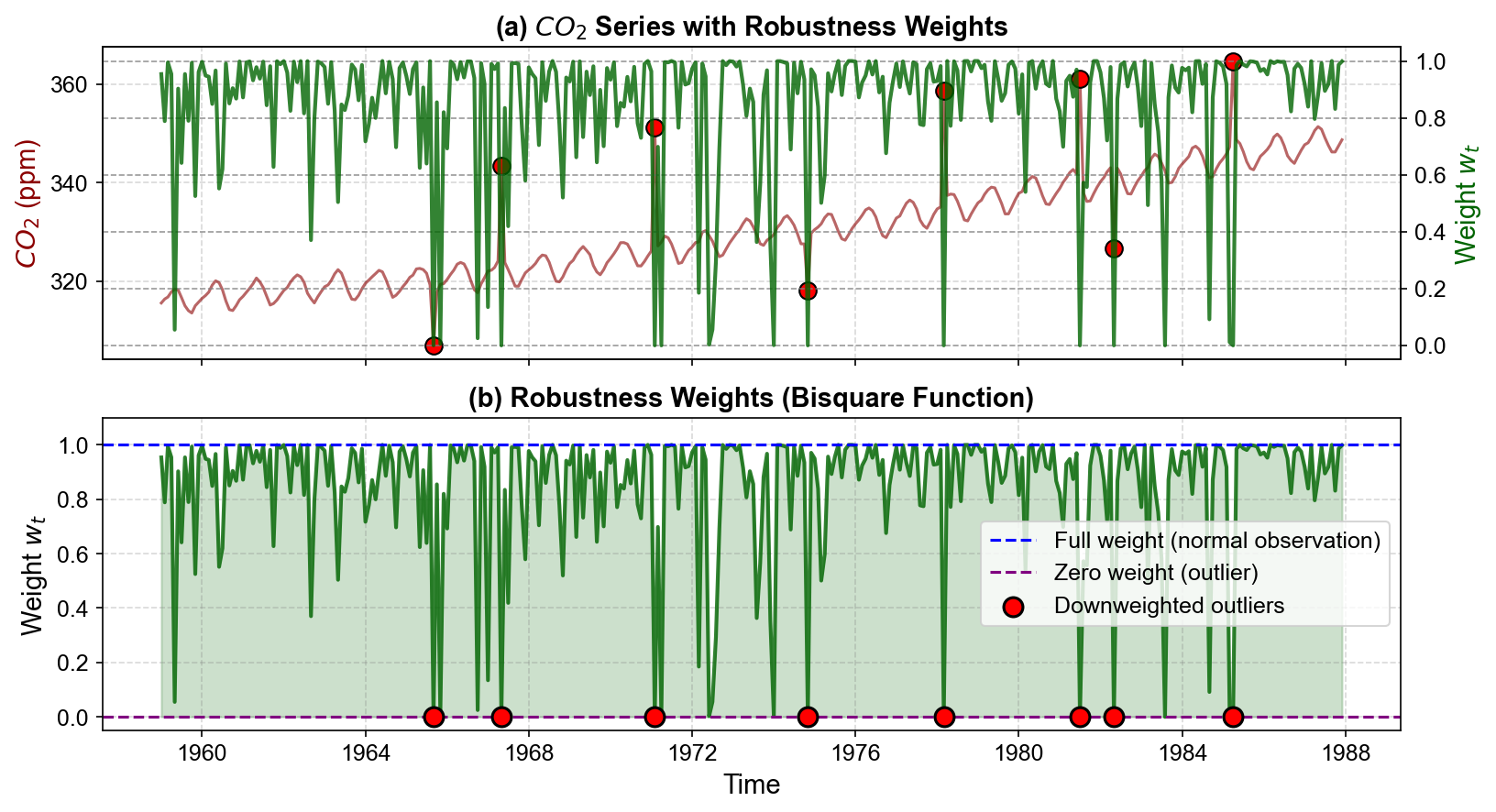
../_images/robustness_weights_co2.png — Fig. 3.20 **(a)** CO₂ series (red) overlaid with robustness weights (green). Most observations receive full weight ($$w_t = 1$), but outlier locations show dramatic weight reductions. **(b)** Detailed view of robustness weights. The bisquare function smoothly downweights deviations, with extreme outliers receiving weights near zero. This ensures outliers have minimal influence on trend and seasonal LOESS fits in the next iteration.#

In Fig. 3.20:

Panel (a) overlays the robustness weights (green line) on top of the CO₂ data. Most of the time, the weight stays at 1.0 (full weight), meaning normal observations are fully trusted. But at each outlier location, the weight drops dramatically—often all the way to zero.
Panel (b) provides a detailed view of just the weights. The algorithm has automatically identified our synthetic outliers and assigned them weights near zero. This is remarkable: we never told the algorithm where the outliers were—it figured it out by itself through the iterative reweighting process.

=== Robustness Weights at Outlier Locations ===
1967-05: w_t = 0.000000
1971-02: w_t = 0.000000
1978-03: w_t = 0.000000
1981-07: w_t = 0.000000
1985-04: w_t = 0.000000
1965-09: w_t = 0.000000
1974-11: w_t = 0.000000
1982-05: w_t = 0.000000

All 8 of our synthetic outliers received weights of exactly 0.000000, meaning they were completely excluded from the trend and seasonal LOESS fits after the first iteration. This automatic outlier detection is a powerful feature of Robust STL.

3.4.4.3. Quantitative Comparison: CO₂ Example#

It’s one thing to see visual differences, but we should also quantify how much better Robust STL performs. The table below summarizes key metrics:

Table 3.7 Quantitative comparison of standard versus robust STL on CO₂ data with synthetic outliers. Robust STL achieves lower residual variance and superior performance on clean data points.#
Metric	Standard STL	Robust STL
Residual Std (All)	2.3778	2.772
Residual Std (Excluding outliers)	1.019	0.2275
Trend Variance	99.8595	98.0299
Seasonal Variance	5.7404	3.9779
Max	Residual

Table 3.7 shows that, when all observations are included, Robust STL has a slightly larger residual standard deviation than the standard STL (2.77 vs 2.38 ppm). This happens because the robust version deliberately refuses to bend the trend and seasonal components toward the extreme outliers, so those points remain as large residuals rather than being partially absorbed.

The second row is the most informative for model quality: after removing the eight outlier timestamps, the residual standard deviation drops from 1.02 ppm under standard STL to 0.23 ppm under Robust STL. This is a drastic improvement in how well the decomposition fits the “normal” part of the series, and it shows that downweighting outliers allows the method to capture the underlying signal much more accurately.

The trend and seasonal variances change only slightly between the two methods (roughly 2% lower trend variance and 31% lower seasonal variance for Robust STL), which indicates that the robust reweighting does not fundamentally distort the long‑term trend or the recurring seasonal cycle. Instead, it mainly cleans up the noise around them.

Finally, the maximum absolute residual is larger for Robust STL (24.35 vs 19.10 ppm). This is actually desirable in this context: because robust STL does not attempt to “explain away” the outliers through the smooth components, those points stand out as very large residuals. That clear separation makes the outliers easier to detect and diagnose, while leaving the bulk of the series well behaved.

3.4.5. Example 2: Financial Data (Electrical Equipment Orders)#

Now the focus shifts from a controlled, synthetic example to a real-world series that contains a genuine economic shock: the 2008–2009 financial crisis. This example illustrates how robust STL behaves when the goal is to extract a stable trend and seasonal pattern from data that include a short but severe collapse.

3.4.5.1. Dataset context#

The electrical equipment manufacturing index (1996–2012) [Statsmodels Developers, 2023] tracks orders for industrial electrical equipment, a leading indicator of business investment. This series captures how firms adjust their spending on large, durable equipment in response to macroeconomic conditions.

Over the sample period, the series shows several distinct regimes:

1996–2007: steady expansion Orders rise gradually, reflecting economic growth, automation, and investment in industrial infrastructure. Superimposed on this trend is a clear annual seasonal cycle, with recurring peaks and troughs.
2008–2009: financial crisis During the global financial crisis, orders fall sharply—by roughly 40% from their pre-crisis peak. This drop is abrupt and unusually deep compared with typical cyclical variation.
2010–2012: partial recovery Orders rebound but do not fully return to pre-crisis levels, suggesting a structural shift in demand.

These features make the series an ideal test bed: the crisis period behaves like an extreme but relatively short-lived shock embedded in an otherwise smoother, seasonal series.

Time range: 1996-01 to 2017-05
Number of observations: 257

init_notebook_modetrusted

Loading ITables v2.6.1 from the init_notebook_mode cell... (need help?)

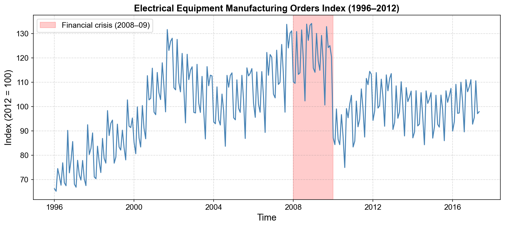
../_images/elec_equip_original.png — Fig. 3.21 Monthly electrical equipment orders index (1996–2012). The series exhibits a clear upward trend and strong seasonality up to 2007, followed by a sharp collapse during the 2008–2009 financial crisis (shaded region) and a partial recovery afterwards. This sudden, deep downturn provides a realistic stress test for STL decomposition methods.#

3.4.5.2. Decomposition: standard vs. robust STL#

To understand how the crisis affects the decomposition, both standard STL and robust STL are applied to the same series using identical seasonal and trend window lengths. The only difference is whether robustness reweighting is enabled.

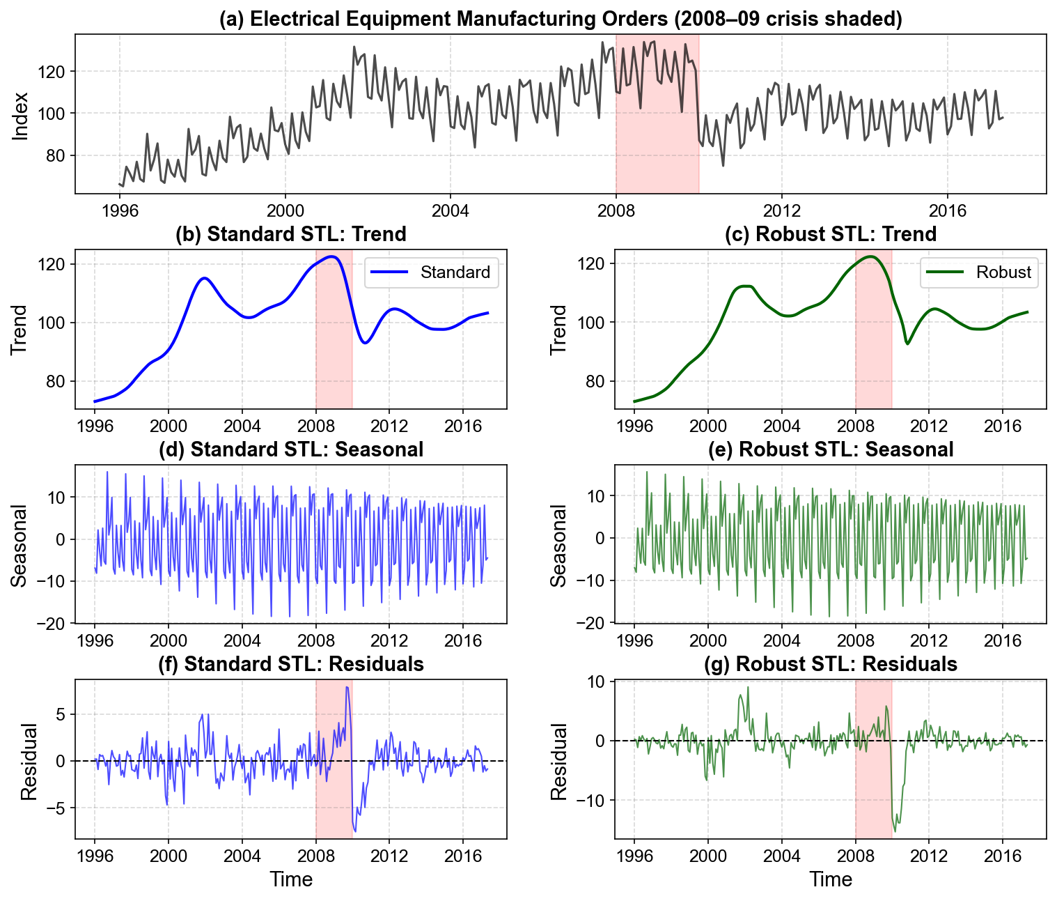
../_images/elec_equip_standard_vs_robust.png — Fig. 3.22 Comparison of standard (left column) versus robust (right column) STL on electrical equipment orders. **(a)** Original series with the 2008–2009 crisis shaded. **(b–c) Trend**: Standard STL (blue) closely follows the crisis collapse, dragging the trend down toward the temporary low and then back up, which can overemphasize a short-lived event. Robust STL (green) yields a smoother trend that acknowledges the downturn but treats it more as a transient shock superimposed on the longer-term trajectory. **(d–e) Seasonal**: Around the crisis years, standard STL’s seasonal component becomes irregular and its amplitude varies noticeably, indicating contamination by the extreme observations. The robust seasonal component remains much more stable, preserving a consistent annual pattern across the full sample. **(f–g) Residuals**: Standard STL shows elevated residuals not only during the crisis but also in neighboring years, suggesting that the shock has “bled” into the fitted components. Robust STL concentrates large residuals mainly within 2008–2009, cleanly isolating the crisis impact in the residual term.#

Visual comparison in Fig. 3.22 highlights the key trade-off. Standard STL tries to fit everything, including rare crises, into the smooth trend and seasonal components. Robust STL instead allows those extreme periods to appear as large residuals, protecting the structure estimated from the more typical months.

3.4.5.3. Robustness weights: how the algorithm “sees” the crisis#

Robust STL implements this behavior through robustness weights. After each iteration, observations with large standardized residuals are assigned lower weights and therefore exert less influence on the next round of trend and seasonal LOESS fits.

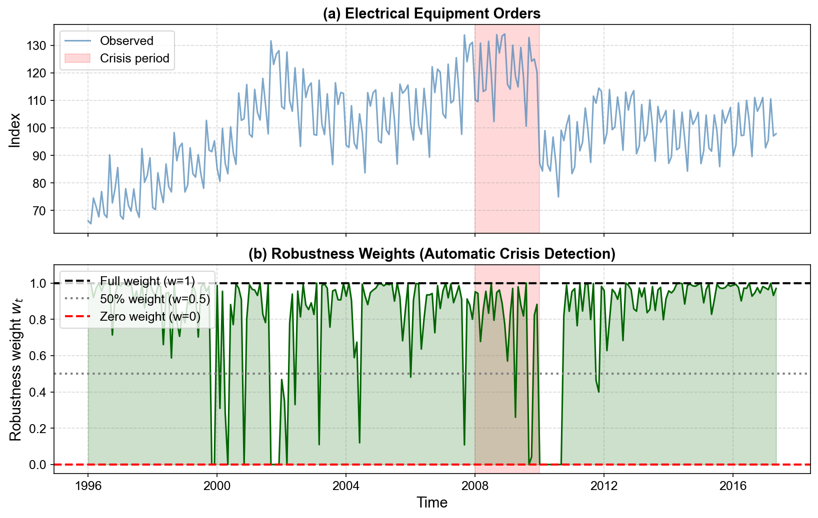
../_images/elec_equip_weights.png — Fig. 3.23 **(a)** Electrical equipment orders with the 2008–2009 crisis shaded. **(b)** Robustness weights (w_t) estimated by the algorithm. For most months, the weight remains near (w_t = 1), meaning these observations fully drive the decomposition. Around the crisis period, however, weights fall sharply—many months are downweighted to (w_t \approx 0.1)–(0.3), and some receive effectively zero weight. A handful of earlier and later months with unusually large spikes or drops are also downweighted. In effect, robust STL automatically flags the crisis and other unusual months as extreme deviations and prevents them from dominating the fitted trend and seasonal components.#

=== Observations with w_t < 0.5 (>50% downweighting) ===
Total: 32 out of 257 months

Downweighted periods:
  1999-11: w_t = 0.0000, Value = 91.33
  1999-12: w_t = 0.0000, Value = 95.27
  2000-02: w_t = 0.3093, Value = 80.58
  2000-04: w_t = 0.2845, Value = 87.12
  2000-05: w_t = 0.0000, Value = 83.33
  2000-11: w_t = 0.0000, Value = 103.37
  2001-09: w_t = 0.0000, Value = 131.65
  2001-10: w_t = 0.0000, Value = 123.06
  2001-11: w_t = 0.0000, Value = 126.82
  2001-12: w_t = 0.0000, Value = 128.08
  2002-01: w_t = 0.4684, Value = 107.71
  2002-02: w_t = 0.3497, Value = 106.85
  2002-03: w_t = 0.0000, Value = 127.59
  2002-06: w_t = 0.3301, Value = 121.84
  2003-03: w_t = 0.1097, Value = 117.34
  2004-06: w_t = 0.1195, Value = 105.12
  2006-01: w_t = 0.4814, Value = 101.28
  2007-09: w_t = 0.1081, Value = 133.79
  2009-04: w_t = 0.2605, Value = 118.76
  2009-09: w_t = 0.0000, Value = 132.86
  2009-10: w_t = 0.0427, Value = 124.22
  2010-01: w_t = 0.0000, Value = 87.05
  2010-02: w_t = 0.0000, Value = 84.31
  2010-03: w_t = 0.0000, Value = 99.01
  2010-04: w_t = 0.0000, Value = 86.54
  2010-05: w_t = 0.0000, Value = 84.30
  2010-06: w_t = 0.0000, Value = 96.67
  2010-07: w_t = 0.0000, Value = 87.68
  2010-08: w_t = 0.0000, Value = 74.90
  2010-09: w_t = 0.0000, Value = 99.16
  2011-10: w_t = 0.4635, Value = 108.97
  2011-11: w_t = 0.3993, Value = 114.45

The printed list of months with $w_t < 0.5$ confirms this behavior. Out of 257 months, only 32 receive more than 50% downweighting. Many of these are clustered in 2009–2010, precisely when orders swing most violently, while a smaller number correspond to earlier isolated spikes and dips. This automatic identification of problematic periods is an important practical advantage: there is no need to hand-label crisis months before running the decomposition.

3.4.5.4. Quantitative Analysis: Financial Crisis Example#

To move beyond visual impressions, the decomposition results are summarized using several metrics, computed separately for the full sample, the non-crisis months, and the crisis window.

Table 3.8 Quantitative comparison of standard versus robust STL on electrical equipment orders. Values summarize residual behavior, and the variability of the trend and seasonal components, for both methods.#
Metric	Standard STL	Robust STL
Residual Std (All data)	2.0529	3.0217
Residual Std (Non-crisis only)	1.8691	3.0767
Residual Std (Crisis only)	2.6926	1.9832
Trend Variance	152.585	149.303
Seasonal Variance	73.3222	69.7763
Max Absolute Residual	7.8961	15.3385

These numbers should be read carefully:

Residual standard deviation (all data). Over the full sample, robust STL has a larger residual standard deviation than standard STL (3.02 vs 2.05). This is expected: the robust method deliberately leaves the crisis months as large residuals instead of smoothing them away, so the overall residual spread increases.
Residual standard deviation (non-crisis months). For months outside the 2008–2009 window, standard STL achieves smaller residuals than the robust version (1.87 vs 3.08). In this dataset, the crisis is not completely isolated in time; the surrounding years remain volatile, and robust STL continues to downweight a number of unusual points. As a result, the non-crisis residuals do not tighten as much as in the synthetic CO₂ example.
Residual standard deviation (crisis months only). Within the crisis window, the story reverses: robust STL has considerably smaller residuals than the standard version (1.98 vs 2.69). Because the robust method allows the trend to decline but resists overfitting individual spikes and troughs, it captures the overall shape of the downturn more cleanly while still treating extreme deviations as outliers.
Trend and seasonal variances. The variances of the trend and seasonal components are slightly lower for robust STL (about 2% lower trend variance and 5% lower seasonal variance). This indicates a modest smoothing effect: robust STL produces slightly less volatile trend and seasonal estimates, consistent with the visual impression of a cleaner decomposition.
Maximum absolute residual. The largest residual under robust STL is almost twice as large as under standard STL (15.34 vs 7.90). This again reflects the design of the robust procedure: rather than spreading the crisis shock across many months and into the smooth components, it leaves a small set of very large residuals. Those months stand out clearly as extreme events, making them easier to identify and interpret.

Taken together, these metrics emphasize that “better” does not simply mean “smaller residuals everywhere.” In settings with rare but important shocks, the goal is often to obtain a stable trend and seasonal pattern while allowing the extreme events to appear explicitly in the residuals. Robust STL prioritizes this separation of structure and shock, which is exactly what is needed for many economic and financial applications.

Summary: practical lessons from the crisis example

This financial crisis example highlights when robust STL is particularly valuable:

When the series contains short-lived but severe disruptions (such as crises, natural disasters, or policy shocks) that should not dominate the long-run trend and seasonal patterns.
When analysts care most about the underlying structure of typical periods, while treating the extremes as events to be studied separately.
When there is a need for automatic downweighting of unusual observations rather than manual pre-screening.

By contrast, if every observation is considered reliable and large moves are viewed as part of the structural evolution of the series—for example, a permanent regime change—then standard STL may be preferable, because it will incorporate those shifts directly into the trend component.

In practice, applying both standard and robust STL side by side, as done here, often provides the most insight: the comparison reveals which parts of the series are fragile to outliers and how much the estimated components depend on a small set of extreme observations.

Residual Size	\(u_t\) Value	Weight \(w_t\)	Interpretation
Normal (Small)	\(u_t = 0\)	\(w_t = 1.00\)	Full Influence (No downweighting)
Moderate	\(u_t = 0.5\)	\(w_t = 0.56\)	Reduced Influence (Partial downweighting)
Outlier Threshold	\(u_t = 1.0\)	\(w_t = 0.00\)	Zero Weight (Completely ignored)
Extreme (Outlier)	\(u_t > 1.0\)	\(w_t = 0.00\)	Completely Excluded