Remark
Please be aware that these lecture notes are accessible online in an ‘early access’ format. They are actively being developed, and certain sections will be further enriched to provide a comprehensive understanding of the subject matter.
5.3. Outlier Classification by Seasonality#
When analyzing time series data with repeating patterns—such as retail sales, energy consumption, or web traffic—an outlier is not simply an “extreme value.” It is a value that defies its seasonal expectation. A data point can be globally normal (e.g., within the overall range of the dataset) yet seasonally anomalous (e.g., far below the expected peak for that time of year).
Classifying outliers based on their relationship to seasonality is critical because it prevents two common errors:
False Positives: Flagging a normal seasonal peak (e.g. December sales) as an outlier just because it is high.
False Negatives: Missing a significant drop in performance (e.g. a poor holiday season) because the value is still higher than an average month.
5.3.1. Why Seasonality Matters#
Consider a retailer analyzing monthly revenue. In December 2024, they record sales of $1.2 million.
Global Perspective: Compared to an average month (e.g., March with $600k), $1.2 million looks fantastic—double the typical revenue.
Seasonal Perspective: Compared to previous Decembers (2022: $2.8M, 2023: $3.1M), $1.2 million is a disaster. It represents a massive underperformance relative to the seasonal norm.
Standard outlier detection methods (e.g. Z-Scores calculated on the entire dataset) would fail here. They might see $1.2M as “high” or “normal,” completely missing the fact that it is an anomaly for December. Effective detection requires methods that decompose the signal into trend, seasonality, and residual components (e.g., STL decomposition) to isolate the true anomalies.
5.3.2. Seasonal Outliers (SO)#
Seasonal outliers are data points that deviate significantly from the expected seasonal pattern. They are anomalous relative to their season, not necessarily relative to the global dataset average.
Characteristics of Seasonal Outliers
Season-Specific: The benchmark is the historical data for that specific period (e.g., compare Dec 2024 only to Dec 2023, Dec 2022…).
Relative Deviation: The anomaly is defined by the gap between the observed value and the expected seasonal peak/trough.
Context-Dependent: A value might be the highest in the dataset yet still be an outlier if it should have been even higher.
Retail Sales: December sales of $1.2M are high globally but low seasonally (expected $2.5M). This indicates a failed holiday campaign or supply chain collapse.
Energy Consumption: January electricity usage of 95,000 kWh is higher than September (80k), but far below the winter norm (150k). This could indicate a broken meter or unusually mild weather.
Web Traffic: A travel site gets 50k visits in July (peak season). If July 2024 sees only 25k visits, it is a seasonal outlier, even if 25k is double the traffic of November.
5.3.2.1. Visualizing Seasonal Anomalies#
Fig. 5.8 illustrates the retail sales scenario. Notice the strong repeating pattern of holiday peaks. The anomaly in December 2024 stands out not because it is small in absolute terms, but because it breaks the established rhythm of the peaks.
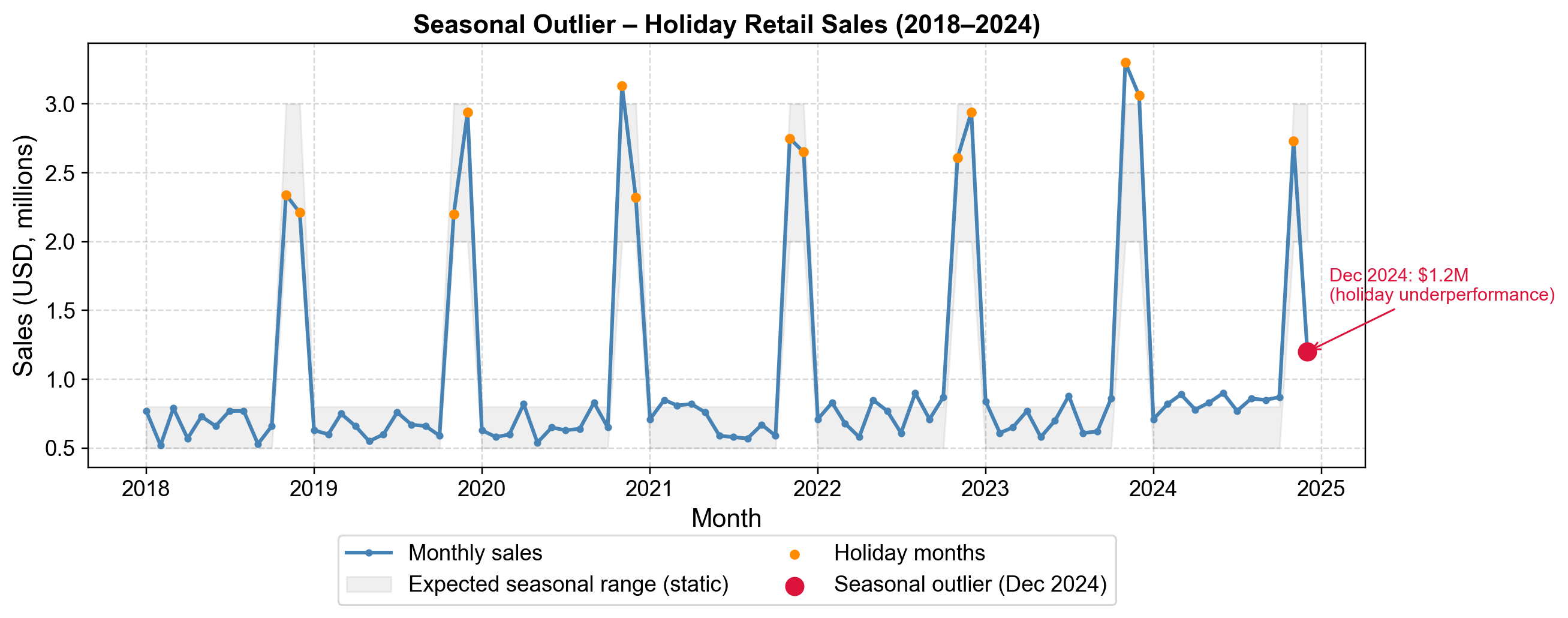
Fig. 5.8 Seasonal Outlier: The “Missing Peak”. The chart tracks monthly retail sales over 7 years. The orange dots highlight the expected holiday peaks (Nov-Dec), which typically reach $2.0–$3.0 million. The red ‘X’ in December 2024 marks a value of $1.2 million. While $1.2M is higher than any non-holiday month (blue dots), it is a massive failure compared to the expected holiday performance. A global outlier detector would likely miss this, seeing it as a “high” value, but a seasonal detector correctly flags it as an anomaly.#
Fig. 5.8 shows monthly retail sales with clear seasonal peaks during November-December (holiday season). The red marker in December 2024 indicates a value of $1.2M. While this exceeds most months throughout the year, it falls dramatically below the typical holiday season performance of $2M–$3M observed in previous years. This seasonal underperformance requires investigation—potential causes include failed marketing campaigns, supply chain disruptions, or changing economic conditions. Detection of this pattern requires seasonal decomposition methods such as STL (Seasonal and Trend decomposition using Loess) or ARIMA-based approaches that model expected seasonal behavior.
5.3.3. Non-Seasonal Outliers#
Non-seasonal outliers are anomalies that exist independently of repeating cycles. Unlike seasonal outliers, which are defined by their deviation from an expected periodic pattern, non-seasonal outliers represent fundamental disruptions to the data generating process itself. They are “pure” anomalies—unexpected events that would be considered outliers regardless of when they occurred.
Characteristics of Non-Seasonal Outliers
Season-Independent: The anomaly is not tied to a specific calendar period (e.g., it is not just a “bad December”).
Universal Deviation: The value is unusual relative to the immediate local trend or the global distribution, not just a seasonal benchmark.
Structural Impact: These often signal external shocks (e.g., policy changes, system failures) rather than cyclical variations.
Classification by Duration: They are typically categorized by how long their impact persists—ranging from a single point to a permanent shift.
5.3.3.1. The Four Types of Temporal Impact#
When a non-seasonal outlier occurs, its most important characteristic is not just its magnitude, but its persistence. Does the system snap back to normal immediately, or does the outlier change the future trajectory? We classify these into four distinct types [Fox, 1972, Tsay, 1988]:
Additive Outliers (AO): A one-time spike that affects a single observation. The system returns to normal immediately (e.g., a data entry error).
Innovational Outliers (IO): A shock to the underlying system that affects the current value and propagates into future values, often decaying over time (e.g., a marketing campaign that boosts sales for several weeks).
Level Shifts (LS): A step-change where the baseline of the series moves to a new level permanently (e.g., a new regulation that permanently lowers production capacity).
Transient Changes (TC): A sudden spike that decays exponentially back to the original baseline (e.g., a natural disaster recovery).
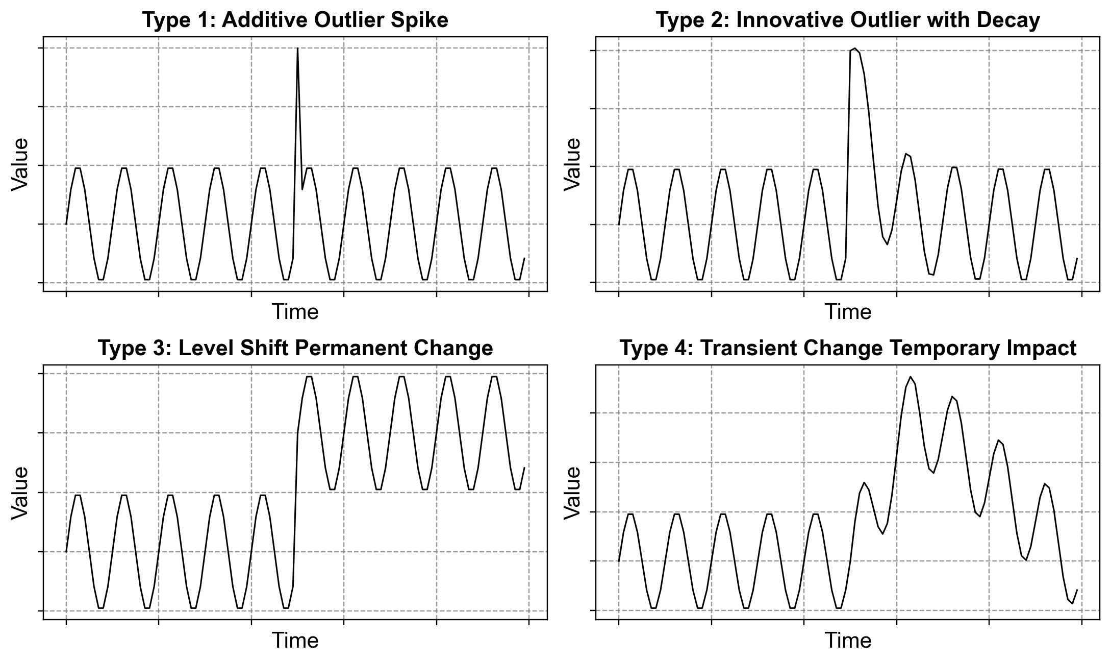
Fig. 5.9 Four types of non-seasonal outliers classified by their temporal impact patterns: (Type 1) Additive outlier showing isolated spike, (Type 2) Innovative outlier with gradual decay, (Type 3) Level shift causing permanent mean change, (Type 4) Transient change with temporary elevation.#
5.3.3.2. Type 1: Additive Outliers (AO) – Isolated Impact#
An additive outlier represents an extraordinary event that affects a single observation only. The effect is completely isolated, and the time series immediately returns to its normal pattern after the outlier. Think of it as a one-off spike that appears and disappears without leaving any trace.
Characteristics of Additive Outliers
Duration: Single time period only
Effect: No impact on subsequent observations
Recovery: Immediate return to baseline
Data Entry Error
A clerk accidentally enters \(50,000 instead of \)5,000 for a single day’s sales
Next day’s sales return to the normal range around $5,000
No lasting impact on the business or data pattern
Momentary Sensor Malfunction
Temperature sensor briefly reads 150°C due to electrical interference
Next reading shows normal 22°C
System and actual temperature remain unaffected
Viral Social Media Spike
A single tweet from a celebrity drives 100,000 website visits in one day
Normal daily traffic averages 5,000 visits
Next day returns to 5,000 with no sustained interest
The mathematical representation of an Additive Outlier is expressed as:
Component Definitions:
\(Y_t'\) = The observed (contaminated) value at time \(t\) that we actually measure
\(Y_t\) = The true underlying value that would exist without any outlier present (the clean, uncontaminated data)
\(\omega_a\) = The additive magnitude or amplitude of the outlier—the fixed amount by which the observation deviates. This can be positive (upward spike) or negative (downward dip)
\(T\) = The specific time index where the outlier occurs (a single, fixed point in time)
\(t\) = Any time point in the series
What This Equation Means:
At the outlier time point \(t = T\), the observed value equals the true value plus an additive shock of magnitude \(\omega_a\). For all other times (\(t \neq T\)), the observed value equals the true value exactly—no contamination occurs before or after the outlier.
Example 5.1
Consider a scenario tracking daily website traffic over 120 days (January to April 2024). The baseline series includes:
A mild upward trend (organic growth of 0.02 units per day)
Weekly seasonality (higher traffic on weekdays, lower on weekends)
Random noise representing daily fluctuations
On Day 75 (March 16, 2024), a system malfunction or data logging error occurs that causes the recorded traffic \(Y_{75}'\) to spike by exactly \(\omega_a = 12.0\) units above the true value \(Y_{75}\).
Mathematical representation:
If the true traffic on Day 75 was \(Y_{75} = 48.5\) visits (baseline), then:
Observed value with outlier: \(Y_{75}' = 48.5 + 12.0 = 60.5\) visits
Day 74 (unaffected): \(Y_{74}' = Y_{74} = 49.2\) visits
Day 76 (unaffected): \(Y_{76}' = Y_{76} = 50.1\) visits
The outlier only contaminates the single observation at Day 75. The day immediately before and after show normal behavior with no lasting impact. The sharp red spike in the visualization clearly illustrates this isolated disturbance—it appears suddenly, deviates significantly from the baseline (gray line), then the series resumes its normal pattern.
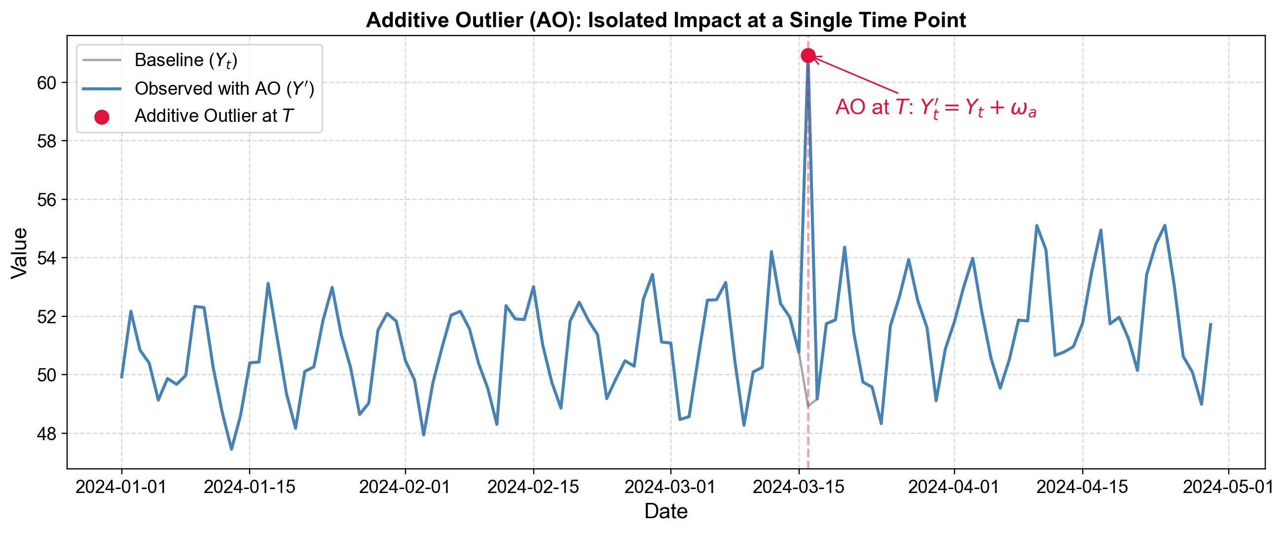
Fig. 5.10 Additive Outlier (AO): Isolated spike at time \(T\) with immediate return to baseline and no lasting effect on subsequent observations.#
The time series shows stable baseline behavior with typical fluctuations. The sharp spike appears suddenly on one day, reaching a value far above the normal range. The critical feature is that the day after the spike, the series immediately returns to its previous baseline level. There is no gradual decay, no shift in the mean, no persistent effect—just an isolated anomaly that affects only a single time point.
5.3.3.3. Type 2: Innovative Outliers (IO) – Decaying Persistence#
An innovative outlier represents an extraordinary event that creates a shock to the underlying system, affecting not just the current observation but also subsequent ones with gradually diminishing impact over time. Unlike an additive outlier’s isolated spike, an innovative outlier leaves a memory in the system that fades exponentially [Chen and Liu, 1993, Lindemann et al., 2021, Vishwakarma et al., 2020].
Characteristics of Innovative Outliers (IO)
Duration: Affects current and multiple future observations
Effect: Persistent but decreasing—strongest at occurrence, then fades
Recovery: Gradual return to baseline over several periods
Successful Marketing Campaign
A major promotional campaign boosts sales from $50K/week baseline in Week 1
Week 1: $150K (initial shock from campaign launch)
Week 2: $90K (elevated but declining—lingering campaign effects)
Week 3: $70K (still above baseline—word-of-mouth continues)
Week 4: $55K (nearly back to normal—momentum dissipates)
The initial shock creates momentum that takes time to dissipate
Viral Content Effect
A viral YouTube video drives 500K website visits on Day 1 (baseline: approximately 10K)
Day 2: 200K (still very high—shares continue)
Day 3: 80K (declining—algorithm stops prioritizing)
Day 4: 30K (approaching normal)
Day 7: 12K (back to baseline of approximately 10K)
The viral effect gradually wears off as momentum decays
Product Launch
New smartphone model creates demand shock on launch
Week 1: Initial rush of early adopters (baseline plus 200%)
Week 2-4: Word-of-mouth drives continued elevated demand (declining each week)
Week 5-8: Demand slowly stabilizes back to baseline
The launch event triggers a lingering effect that gradually vanishes
The mathematical representation of an Innovative Outlier is expressed as:
where the decay function is:
Component Definitions:
\(Y_t'\) = The observed (contaminated) value at time \(t\)
\(Y_t\) = The true underlying value without the outlier
\(\omega_i\) = The initial shock magnitude at time \(T\)—the maximum additive impact at the moment the event occurs
\(\psi_{t-T}\) = The decay function that controls how the shock effect diminishes over time
\(\phi\) = The decay factor (\(0 < \phi < 1\)), which determines how quickly the impact fades
\(\phi = 0.9\): Slow decay (effect lingers a long time)
\(\phi = 0.7\): Moderate decay (effect fades in weeks)
\(\phi = 0.5\): Fast decay (effect mostly gone in a few periods)
\(T\) = The time index when the shock event occurs
\(t - T\) = The number of periods since the shock
What This Equation Means:
At time \(T\), the outlier injects a full shock of magnitude \(\omega_i\). As time progresses beyond \(T\), the shock’s influence is multiplied by the decay function \(\psi_{t-T} = \phi^{t-T}\), which shrinks exponentially. The effect never completely disappears mathematically, but becomes negligible after several periods.
For example, with \(\phi = 0.85\):
At \(t = T\) (Day 0): Impact = \(0.85^0 \times \omega_i = 1.0 \times \omega_i\) (full shock)
At \(t = T+1\) (Day 1): Impact = \(0.85^1 \times \omega_i = 0.85 \times \omega_i\) (85% remaining)
At \(t = T+2\) (Day 2): Impact = \(0.85^2 \times \omega_i = 0.72 \times \omega_i\) (72% remaining)
At \(t = T+5\) (Day 5): Impact = \(0.85^5 \times \omega_i = 0.44 \times \omega_i\) (44% remaining)
At \(t = T+10\) (Day 10): Impact = \(0.85^{10} \times \omega_i = 0.20 \times \omega_i\) (20% remaining)
:label: example_innovative_outlier
Consider a scenario tracking daily website traffic over 150 days (January to May 2024). The baseline series includes:
A mild upward trend (organic growth of 0.015 units per day)
Weekly seasonality (higher traffic on weekdays, lower on weekends)
Random noise representing daily fluctuations
On Day 70 (March 11, 2024), a successful viral marketing campaign launches that creates an initial shock of \(\omega_i = 10.0\) additional visits. However, unlike a data entry error (which affects only one day), this campaign’s effect decays gradually with decay factor \(\phi = 0.85\).
Mathematical representation:
If the baseline traffic on Day 70 was \(Y_{70} = 62.5\) visits, then:
Day 70 (shock event at T): \(Y_{70}' = 62.5 + (0.85^0 \times 10.0) = 62.5 + 10.0 = 72.5\) visits
Day 71 (one day later): \(Y_{71}' = Y_{71} + (0.85^1 \times 10.0) = Y_{71} + 8.5\) visits
Day 72: \(Y_{72}' = Y_{72} + (0.85^2 \times 10.0) = Y_{72} + 7.2\) visits
Day 75 (5 days later): \(Y_{75}' = Y_{75} + (0.85^5 \times 10.0) = Y_{75} + 4.4\) visits
Day 80 (10 days later): \(Y_{80}' = Y_{80} + (0.85^{10} \times 10.0) = Y_{80} + 2.0\) visits
The outlier’s effect does not vanish after one day like an additive outlier. Instead, it persists and gradually decays—each day the additional impact is 85% of the previous day’s impact. After approximately 10 days, the campaign’s effect has diminished to just 20% of its original shock value, but it continues to fade slowly.
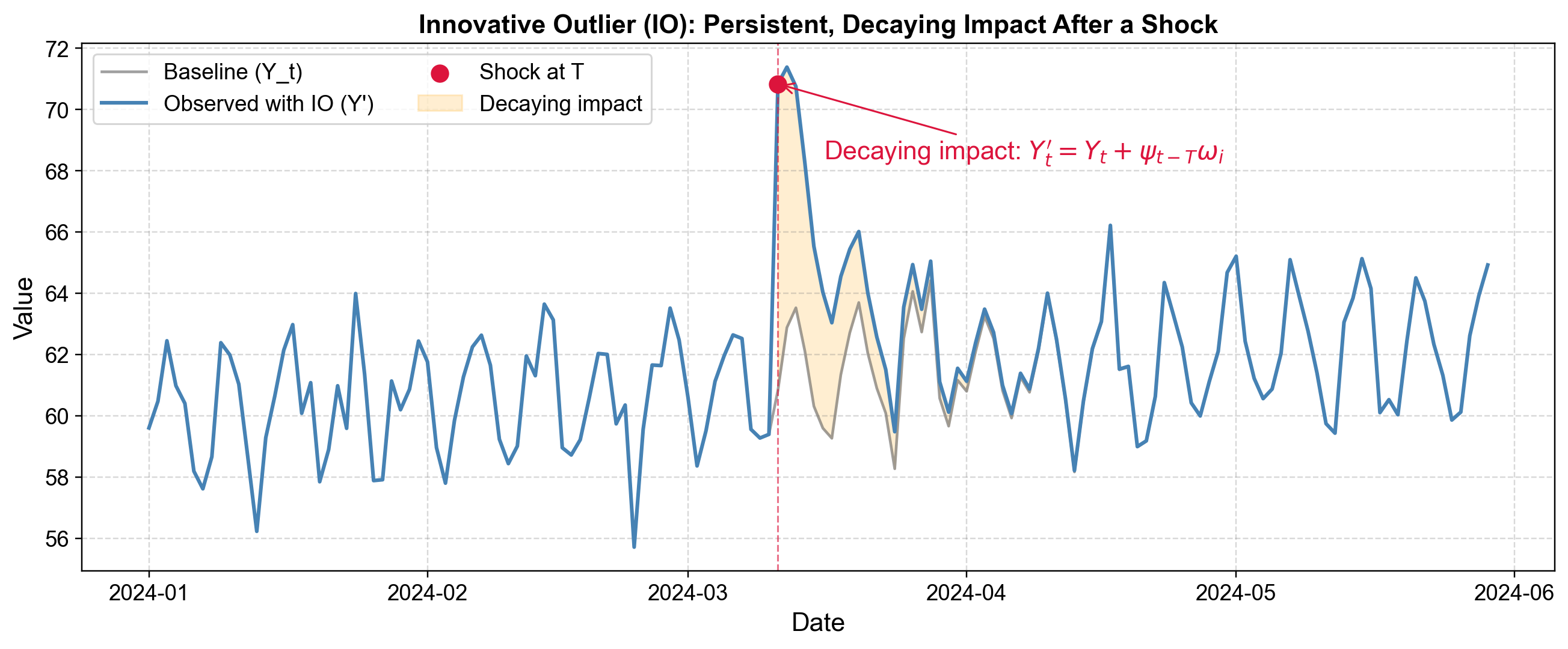
Fig. 5.11 Innovative Outlier (IO): Shock with exponentially decaying persistence over multiple time periods.#
The figure shows the difference between baseline behavior (gray line) and the observed data with the innovative outlier (blue line). The sharp upward shift begins at Day 70 when the campaign launches. Rather than returning to baseline the next day, the series gradually descends back toward the baseline in an exponential decay pattern. The orange shaded area between the two lines represents the persistent impact zone—notice how its width shrinks as days pass, illustrating the decaying nature of the effect.
The initial shock appears as a dramatic spike above baseline. However, unlike an additive outlier, the series does not immediately return to the previous level. Instead, you observe a gradual decay pattern—each subsequent observation is closer to the baseline than the previous one, creating an exponential decay curve back to normal. The system has been perturbed and takes time to settle. The gap between the observed and baseline values shrinks in a smooth, mathematically predictable way rather than dropping sharply.
5.3.3.4. Type 3: Level Shift (LS) – Permanent Structural Change#
A level shift represents an abrupt and permanent change in the mean level of the time series. After the shift occurs, the series stabilizes at a new baseline that persists indefinitely. Unlike an innovative outlier that decays, a level shift represents a structural break where the underlying system itself has changed [Chen and Liu, 1993, Truong et al., 2020].
Characteristics of Level Shift (LS)
Duration: Permanent, indefinite persistence
Effect: Constant long-term impact on series level
Recovery: No recovery—the change is permanent
Pattern: Step function—immediate jump to new mean level
Retail Store Expansion
Company operates at baseline revenue of $500K/month
After opening 10 new store locations, immediate jump occurs
Post-expansion: $1.2M/month (permanent new baseline)
Revenue remains elevated indefinitely—no decay back to original level
The structural change in business capacity creates a permanent revenue increase
New Government Regulation
Environmental tax implemented on manufacturing
Pre-tax production cost: $80/unit (baseline)
Post-tax implementation: $95/unit (permanent new cost)
Production costs remain elevated indefinitely due to policy change
Once the tax is in place, costs do not gradually return to previous levels
Company Merger
Company A (revenue: $5M/quarter) merges with Company B (revenue: $3M/quarter)
Pre-merger: $5M/quarter baseline
Post-merger: $8M/quarter (new permanent baseline)
Combined entity operates at structurally higher revenue level indefinitely
Technology Implementation
Factory implements automation system, reducing production time per unit
Pre-automation baseline: 100 units/day
Post-automation: 250 units/day (permanent efficiency gain)
Operational capacity remains elevated—the automation does not wear off
Productivity increase is structural, not temporary
The mathematical representation of a Level Shift is expressed as:
Component Definitions:
\(Y_t'\) = The observed value at time \(t\)
\(Y_t\) = The true underlying value without the shift
\(\omega_{ls}\) = The level shift magnitude—the permanent, fixed amount by which the entire series level changes. This remains constant for all \(t \geq T\)
\(T\) = The time index when the structural shift occurs (the change point)
\(t\) = Any time point in the series
What This Equation Means:
Before the shift time \(t = T\), the observed value equals the true value (no contamination). At \(t = T\) and for all subsequent times \(t > T\), the observed value equals the true value plus a constant, permanent additive amount \(\omega_{ls}\). This shift never decays, never changes—it represents a permanent structural alteration to the system’s baseline level.
The key distinction from other outlier types:
Additive Outlier (AO): Affects only \(t = T\), then disappears
Innovative Outlier (IO): Affects \(t \geq T\) but decays exponentially over time
Level Shift (LS): Affects \(t \geq T\) with constant magnitude forever—no decay
For example, with a shift magnitude \(\omega_{ls} = 8.0\) occurring at \(T = 100\):
At \(t = 99\) (before shift): \(Y_{99}' = Y_{99}\) (no offset)
At \(t = 100\) (shift occurs): \(Y_{100}' = Y_{100} + 8.0\) (offset appears)
At \(t = 101\): \(Y_{101}' = Y_{101} + 8.0\) (same offset persists)
At \(t = 200\): \(Y_{200}' = Y_{200} + 8.0\) (offset unchanged, even 100 periods later)
Example 5.2
Consider a scenario tracking daily production output over 200 days (January to July 2024). The baseline series includes:
A small upward trend (organic efficiency gains of 0.01 units/day)
Weekly seasonality (lower output on Mondays, higher on Thursdays)
Random noise representing daily operational variability
On Day 100 (April 10, 2024), the company implements a new automation system that permanently increases production capacity. This creates a level shift of \(\omega_{ls} = 8.0\) units—production immediately jumps and stays at this elevated level.
Mathematical representation:
If the baseline production on Day 100 was \(Y_{100} = 82.5\) units, then:
Day 99 (before automation): \(Y_{99}' = Y_{99} = 81.2\) units (no shift)
Day 100 (automation implemented at T): \(Y_{100}' = 82.5 + 8.0 = 90.5\) units (shift occurs)
Day 101 (one day later): \(Y_{101}' = Y_{101} + 8.0\) units (offset persists)
Day 150 (50 days later): \(Y_{150}' = Y_{150} + 8.0\) units (still elevated by same amount)
Day 200 (100 days later): \(Y_{200}' = Y_{200} + 8.0\) units (offset remains unchanged)
Unlike an innovative outlier that decays back toward the original baseline, or an additive outlier that affects only a single day, this level shift permanently alters the series level. The production output remains 8.0 units higher every single day for the rest of the observation period—and would continue indefinitely. There is no recovery to the original level; the structural change is permanent.
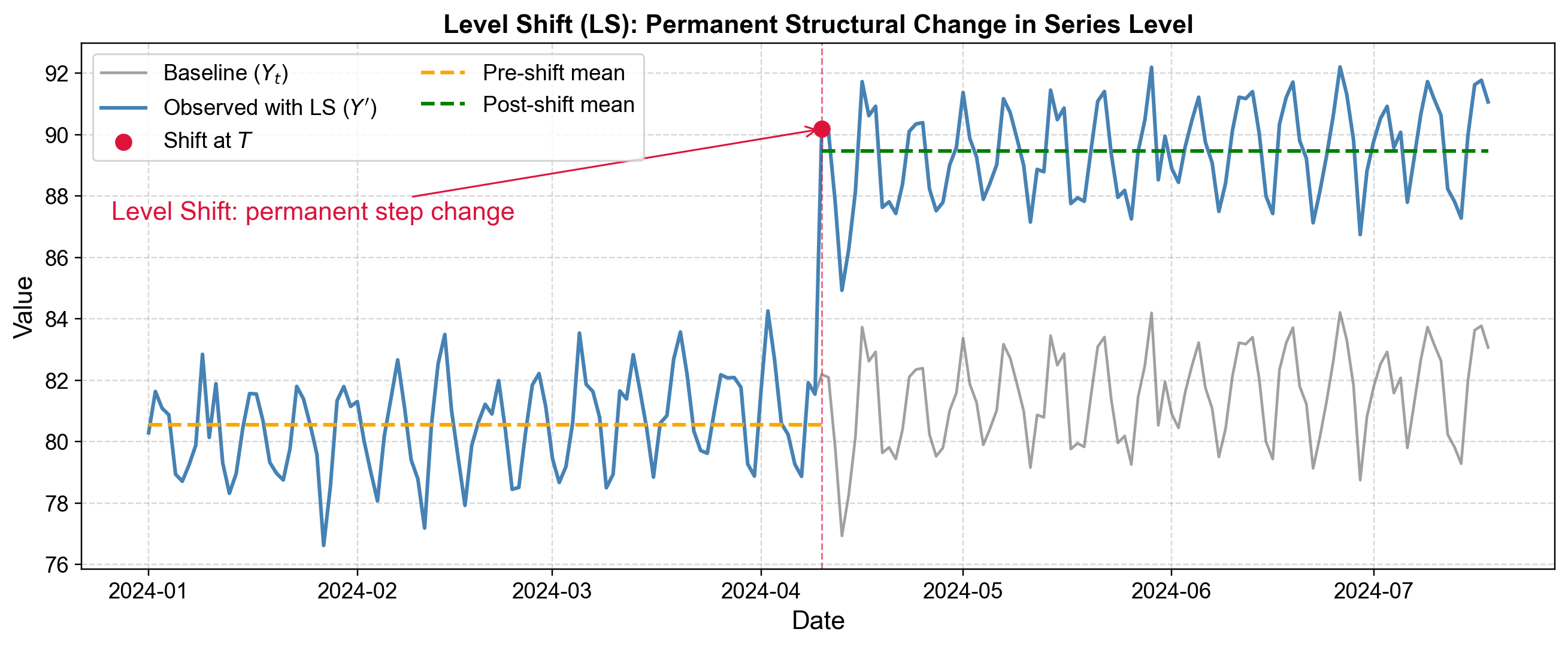
Fig. 5.12 Level Shift (LS): Permanent step change in mean level with no return to baseline.#
The figure clearly shows the difference between baseline behavior (gray line) and the observed data with the level shift (blue line). Before Day 100, both lines fluctuate around the same baseline level. At Day 100 (marked by the vertical red dashed line), the observed series immediately jumps upward. After the jump, the series does not drift back downward—instead, it continues to fluctuate around a permanently elevated mean level (shown by the green dashed line). The orange dashed line represents the pre-shift mean, illustrating how the mean has permanently increased. The constant vertical distance between baseline and observed post-shift demonstrates the persistent, unchanging nature of \(\omega_{ls}\).
Before the change point, the series fluctuates around one stable baseline level. At a specific change point, there is a sharp, immediate jump. After the change point, the series fluctuates around a new, higher (or lower) baseline with no tendency to return to the previous level. The sections before and after appear like two separate time series at different mean levels. Unlike a decaying outlier where the gap shrinks over time, the gap between pre-shift and post-shift levels remains constant—the shift is truly structural and permanent.
5.3.3.5. Type 4: Transient Change (TC) – Temporary Structural Change#
A transient change represents a temporary structural change similar to a level shift, but its effect gradually decays over time rather than being permanent. The series initially experiences a shock or shift, then slowly drifts back to its original baseline. This can be understood as a temporary new normal that eventually fades away [Chen and Liu, 1993, Tsay, 1988, Vishwakarma et al., 2020].
Characteristics of Transient Change (TC)
Duration: Temporary with exponential decay
Effect: Initial impact resembles a level shift, then gradual return
Recovery: Exponential decay back to baseline
Pattern: Step change, then smooth exponential decay downward
Labor Strike
Factory operates at baseline: 1,000 units/day
Strike occurs—immediate drop to 200 units/day
Strike ends but productivity does not immediately recover
Week 1 post-strike: 400 units/day (still impaired)
Week 2: 600 units/day (improving)
Week 4: 900 units/day (nearly recovered)
Week 6: 1,000 units/day (full recovery)
The impact decays gradually as production ramping accelerates
Supply Chain Disruption
Hurricane damages supplier facility, forcing use of expensive alternative suppliers
Unit cost jumps from \(50 to \)80 (immediate impact)
As supplier rebuilds and resumes production:
Month 1: $75/unit (partial recovery)
Month 2: $62/unit (improving)
Month 3: $52/unit (nearly back)
Month 4: $50/unit (fully recovered)
The cost advantage from the normal supplier gradually returns
Seasonal Marketing Campaign
Major holiday advertising campaign boosts sales temporarily
Campaign ends, but brand awareness and momentum linger
Sales remain elevated for several weeks post-campaign
Gradually decay back to baseline as brand recall fades naturally
Unlike permanent level shifts, the effect is truly temporary
Weather Event Impact
Severe winter storm disrupts retail operations
Sales drop 60% during storm week (initial shock)
Recovery is gradual as store repairs, restocking, and customer confidence return
Week 1 post-storm: 50% of baseline (still recovering)
Week 2: 75% of baseline (improving)
Week 4: 95% of baseline (nearly normal)
Takes 3-4 weeks to fully return to normal sales patterns
The mathematical representation of a Transient Change is expressed as:
where the decay function is:
Component Definitions:
\(Y_t'\) = The observed value at time \(t\)
\(Y_t\) = The true underlying value without the transient change
\(\omega_{tc}\) = The initial magnitude of the transient change at \(t = T\)—the immediate shock size
\(\psi_{t-T}\) = The decay function that controls how the transient effect diminishes
\(\delta\) = The decay factor (\(0 < \delta < 1\)), which determines the rate of recovery
\(\delta = 0.95\): Very slow decay (effect lingers for months)
\(\delta = 0.80\): Moderate decay (effect fades over weeks)
\(\delta = 0.60\): Faster decay (effect largely gone in 10-15 days)
\(\delta = 0.30\): Very fast decay (effect nearly gone in a few days)
\(T\) = The time index when the transient event occurs (the onset point)
\(t - T\) = The number of periods since the transient change began
What This Equation Means:
Before time \(T\), the observed value equals the true value (no disturbance). At \(t = T\), the transient change begins with full magnitude \(\omega_{tc}\). Unlike a level shift that remains constant, the transient effect decays exponentially through the function \(\psi_{t-T} = \delta^{t-T}\). As time progresses, the observed value gradually approaches the baseline again. Mathematically, the effect approaches zero asymptotically but never quite disappears.
Comparison with Other Outlier Types:
Additive Outlier (AO): \(Y_T' = Y_T + \omega_a\), then \(Y_{T+1}' = Y_{T+1}\) (disappears immediately)
Innovative Outlier (IO): Similar decay form as TC, but the decay represents system memory effects
Level Shift (LS): \(Y_t' = Y_t + \omega_{ls}\) for all \(t \geq T\) (constant, no decay)
Transient Change (TC): Combines level shift’s initial step with exponential decay (temporary structural change)
For example, with initial impact \(\omega_{tc} = 9.0\) and decay factor \(\delta = 0.80\) occurring at \(T = 60\):
At \(t = 60\) (onset): Impact = \(0.80^0 \times 9.0 = 9.0\) (full initial impact)
At \(t = 61\): Impact = \(0.80^1 \times 9.0 = 7.2\) (80% of initial)
At \(t = 62\): Impact = \(0.80^2 \times 9.0 = 5.76\) (64% of initial)
At \(t = 65\): Impact = \(0.80^5 \times 9.0 = 2.95\) (33% of initial)
At \(t = 75\): Impact = \(0.80^{15} \times 9.0 = 0.34\) (4% of initial)
Example 5.3
Consider a scenario tracking daily retail sales over 180 days (January to June 2024). The baseline series includes:
A small upward trend (seasonal growth of 0.012 units/day)
Weekly seasonality (higher sales on weekends, lower on Mondays)
Random noise representing daily customer variability
On Day 60 (March 1, 2024), a major supply chain disruption occurs—a hurricane damages the primary supplier facility. This forces the company to use more expensive alternative suppliers, creating an initial shock of \(\omega_{tc} = 9.0\) in daily unit costs. However, as the primary supplier rebuilds and resumes operations, the disruption’s effect gradually decays with factor \(\delta = 0.80\).
Mathematical representation:
If the baseline cost per unit on Day 60 was \(Y_{60} = 70.0\), then:
Day 59 (before disruption): \(Y_{59}' = Y_{59} = 70.0\) (no change)
Day 60 (disruption onset at T): \(Y_{60}' = 70.0 + (0.80^0 \times 9.0) = 70.0 + 9.0 = 79.0\) (full impact)
Day 61 (one day later): \(Y_{61}' = Y_{61} + (0.80^1 \times 9.0) = Y_{61} + 7.2\) (80% of impact remains)
Day 62: \(Y_{62}' = Y_{62} + (0.80^2 \times 9.0) = Y_{62} + 5.76\) (64% of impact)
Day 65 (5 days later): \(Y_{65}' = Y_{65} + (0.80^5 \times 9.0) = Y_{65} + 2.95\) (only 33% remains)
Day 75 (15 days later): \(Y_{75}' = Y_{75} + (0.80^{15} \times 9.0) = Y_{75} + 0.34\) (only 4% remains)
The transient change creates an initial spike that resembles a level shift—costs jump from 70 to 79. However, unlike a permanent level shift, the excess cost gradually declines. By Day 75 (two weeks after the event), the disruption’s effect has diminished to nearly nothing, and the series has recovered most of the way back to its original baseline. The recovery follows an exponential decay pattern rather than remaining stuck at the elevated level or returning immediately.
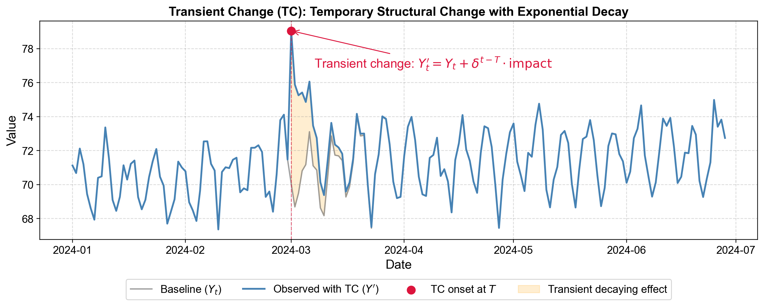
Fig. 5.13 Transient Change (TC): Temporary structural change with gradual exponential decay back to baseline.#
The figure shows the behavior of a transient change. Before Day 60 (marked by the vertical red dashed line), the baseline (gray line) and observed series (blue line) are identical. At Day 60, the observed series jumps upward due to the disruption—resembling a level shift. However, the series does not stay at this elevated level. Instead, the orange shaded area between the baseline and observed lines gradually shrinks, indicating the decaying nature of the transient effect. The observed series curves back toward the baseline in an exponential decay pattern, eventually approaching it asymptotically.
The series shows a sudden step change (upward or downward) similar to a level shift. However, unlike a level shift that permanently stays at the new level, you observe a gradual drift back toward the original baseline. The recovery is not immediate like an additive outlier, and it is not a continuous decay from the shock point like an innovative outlier. Instead, the series appears to step to a new level momentarily, then slowly recover from that temporarily elevated (or depressed) state. The gap between observed and baseline systematically shrinks over time in an exponential decay pattern.
5.3.4. Distinguishing Among Outlier Types#
The critical feature that distinguishes these four outlier types is their temporal fingerprint—the pattern of influence they exert on observations following the initial event. Understanding these distinctions is essential for proper model specification and accurate forecasting.
5.3.4.1. Temporal Signatures#
Each outlier type creates a distinct pattern in the time series post-event:
Additive Outliers affect only the observation at time \(T\), with no influence on subsequent values. The series returns to its baseline immediately, creating an isolated spike that appears disconnected from the surrounding pattern.
Innovative Outliers create a shock that propagates through the system’s autoregressive structure. The effect diminishes exponentially according to the decay parameter \(\phi\), with each subsequent observation carrying a fraction of the previous period’s impact. The visual pattern resembles a sharp initial spike followed by a curved, smooth decline back to baseline.
Level Shifts introduce a permanent change in the series mean. All observations at \(t \geq T\) are shifted by a constant amount \(\omega_{ls}\), creating a clear step function in the data. The pre-shift and post-shift segments appear as two distinct processes operating at different mean levels.
Transient Changes combine characteristics of level shifts and innovative outliers. The series experiences an initial step change at time \(T\), but unlike a permanent level shift, the deviation decays exponentially. This creates a plateau-like pattern where the series temporarily operates at an elevated (or depressed) level before gradually returning to baseline.
5.3.4.2. Implications for Time Series Analysis#
The distinction among these outlier types has direct consequences for model identification, parameter estimation, and forecasting accuracy. Chen and Liu (1993) demonstrated that misclassifying outlier types can lead to severely biased parameter estimates in ARIMA models and degraded forecast performance [Chen and Liu, 1993].
When a level shift is incorrectly treated as an additive outlier and removed from the data, the model will consistently underpredict (or overpredict) all future values because it fails to recognize the structural change in the process mean. Conversely, treating a transient change as a permanent level shift will lead to forecast errors that persist long after the transient effect has dissipated.
The temporal pattern also provides diagnostic information about the underlying cause. Additive outliers typically result from measurement errors, data entry mistakes, or brief equipment malfunctions that do not affect the actual system state. Level shifts indicate fundamental structural changes—policy interventions, technological implementations, or business model changes that permanently alter system behavior. Innovative and transient outliers often arise from external shocks that temporarily disturb the system but do not permanently change its fundamental dynamics.
5.3.4.3. Detection Strategy Considerations#
Accurate outlier classification requires methods that can distinguish among these temporal patterns. Simple threshold-based approaches that only examine the magnitude of deviations at individual time points cannot distinguish an additive outlier from the initial observation of a level shift. Both appear as extreme values at time \(T\), but they require completely different modeling responses.
Effective detection algorithms must evaluate not just the magnitude of deviation at a single point, but the pattern of residuals in the neighborhood surrounding the candidate outlier. The iterative outlier detection procedure proposed by Chen and Liu (1993) [Chen and Liu, 1993] and implemented in various statistical software packages tests for each outlier type simultaneously by fitting intervention models and comparing likelihood ratios. Change-point detection algorithms such as PELT (Pruned Exact Linear Time) [Haynes et al., 2017] and Binary Segmentation can identify level shifts by detecting abrupt changes in distributional parameters.
For seasonal time series, proper decomposition into trend, seasonal, and residual components is essential before applying outlier detection. STL (Seasonal and Trend decomposition using Loess) and X-13-ARIMA-SEATS provide robust frameworks for separating these components, allowing outlier detection methods to operate on the deseasonalized residuals where deviations from expected patterns become more apparent.
5.3.4.4. Forecasting Implications#
The choice of how to handle each outlier type directly impacts forecast accuracy. Additive outliers should be replaced with interpolated values or treated as missing data during model estimation to prevent them from distorting parameter estimates. Level shifts require updating the model structure to include an intervention variable that captures the permanent change in mean level. Innovative and transient outliers may require explicit modeling through transfer functions that capture the temporal dynamics of the shock’s decay.
Ignoring these distinctions leads to systematic forecast errors. Forecasts from models that fail to account for level shifts will exhibit persistent bias, while models that inappropriately retain additive outliers will show inflated residual variance and wider prediction intervals than warranted.