Remark

Please be aware that these lecture notes are accessible online in an ‘early access’ format. They are actively being developed, and certain sections will be further enriched to provide a comprehensive understanding of the subject matter.

2.2. Identifying Patterns of Missingness

2.2.1. Identifying Missing Values

In pandas, we can utilize the isna() or isnull() methods to identify missing values. Both methods function identically and can be used interchangeably to detect NaN (Not a Number) entries in the dataset.

2.2.2. Example: Mississippi River Gage Height Data

To analyze the distribution of missing values over time for the Mississippi River at Thebes, IL dataset, focusing on the ‘77623_00065’ variable (which represents gage height):

The dataset for the Mississippi River at Thebes, IL was analyzed to examine the distribution of missing values in the gage height (ft) variable over time. The data was processed to ensure a complete 30-minute interval time series, allowing us to identify and visualize missing values effectively.

1. Data Ingestion and Cleaning: First, we isolate the timestamp and gage-height fields, standardize names, and enforce a unique, chronological index.

Show code cell source

Hide code cell source

import pandas as pd

# Load only datetime and the raw gage-height column
df = pd.read_csv(
    'chapter02_data/07022000.csv',
    usecols=['datetime', '77623_00065'],
    parse_dates=['datetime']
)

# Rename for readability
df.rename(columns={'77623_00065': 'gage height (ft)'}, inplace=True)

# Remove duplicate timestamps (keep first measurement)
df = df.drop_duplicates(subset='datetime').set_index('datetime').sort_index()

Eliminating duplicates ensures each timestamp corresponds to at most one measurement, avoiding artificial clustering or gaps.

2. Constructing a Continuous 30-Minute Time Base: To clearly identify missing observations, we generate every half-hour timestamp between the earliest and latest recorded times, then reindex.

Show code cell source

Hide code cell source

# Generate full 30-minute interval index
full_index = pd.date_range(
    start=df.index.min(),
    end=df.index.max(),
    freq='30min'
)

# 2Reindex, introducing NaNs where measurements are missing
df = df.reindex(full_index)

This step turns absent timestamps into explicit NaN values in gage_height_ft, making gaps instantly visible and quantifiable.

3. Quantifying Overall Missingness: We compute both the raw count and the percentage of missing gage-height readings.

Show code cell source

Hide code cell source

total_points = len(df)
missing_count = df['gage height (ft)'].isna().sum()
missing_pct = 100 * missing_count / total_points

print(f"Total records: {total_points}")
print(f"Missing measurements: {missing_count} ({missing_pct:.2f}%)")

Total records: 17520
Missing measurements: 388 (2.21%)

Out of the complete half-hourly series, 388 values are missing, representing 2.21% of all time points.

Now, this dataset looks like the following.

Loading ITables v2.6.2 from the init_notebook_mode cell... (need help?)

2.2.3. Visualizing Missingness Patterns

2.2.3.1. Heatmap of Missing Data

A heatmap (can be found in seaborn library) displays each timestamp (x-axis) against the single variable (y-axis), highlighting missing points in red.

Show code cell source

Hide code cell source

import seaborn as sns
import matplotlib.pyplot as plt


# Create a heatmap
plt.figure(figsize=(10, 4))
sns.heatmap(df.isnull().T, cbar=False, cmap="Reds")
plt.yticks([])
plt.title("Heatmap of Artificially Introduced Missing Values")
plt.tight_layout()

Dense red clusters indicate periods with extended data loss (e.g., sensor outages or transmission failures).

2.2.3.2. Temporal Scatter of Gaps

Plotting each missing timestamp along the time axis clarifies whether missingness is random or concentrated.

Show code cell source

Hide code cell source

import matplotlib.pyplot as plt

# Create a mask for missing values
missing_mask = df['gage height (ft)'].isnull()

# Create the figure and axis
fig, ax = plt.subplots(figsize=(10, 2))

# Plot missing values over time
ax.scatter(df.index[missing_mask], [1] * sum(missing_mask), color='red', alpha=0.5, s=10, marker = "s")
ax.set(title = 'Distribution of Missing Values in Gage Height Over Time',
       xlabel = 'Date',
       ylabel = 'Missing Value',
       yticks = []
       )
plt.tight_layout()

Missing readings appear sporadic with occasional clusters—suggesting Missing Completely At Random (MCAR) for most periods, punctuated by brief outages.

2.2.3.3. Monthly Missingness Bar Chart

Aggregating by month highlights seasonal or operational trends in data availability.

Show code cell source

Hide code cell source

import matplotlib.pyplot as plt

# Calculate percentage of missing values per month
missing_percentage = df['gage height (ft)'].isnull().resample('ME').mean() * 100

# Set the index to month names
missing_percentage.index = missing_percentage.index.strftime('%b %Y')  # E.g., 'Jan 2024'

# Create the figure and axis
fig, ax = plt.subplots(figsize=(10, 5))

# Plot missing percentage over time
missing_percentage.plot(kind='bar', color='red', ec='k', alpha=0.7, ax=ax)

# Customize the plot
ax.set(
    title='Percentage of Missing Values by Month',
    xlabel='Month',
    ylabel='Percentage of Missing Values'
)
ax.tick_params(axis='x', rotation=45)

# Adjust layout and show the plot
plt.tight_layout()

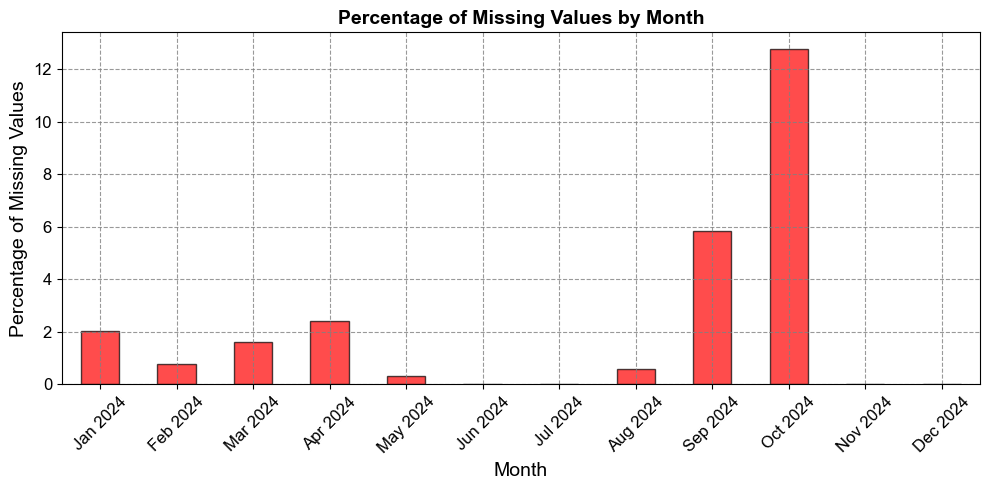
• This visualization highlights periods with higher concentrations of missing data.

• Peaks in the bar chart may correspond to specific months with data collection or transmission issues.

2.2.3.4. Day-of-Year Seasonal Profile

By grouping missingness by day-of-year, we detect recurring annual patterns.

Show code cell source

Hide code cell source

# Aggregate missing values by day of the year
df['day_of_year'] = df.index.dayofyear
seasonal_missing = df.groupby('day_of_year')['gage height (ft)'].apply(lambda x: x.isnull().mean())

# Create the figure and axis
fig, ax = plt.subplots(figsize=(10, 6))
seasonal_missing.plot(color='red', alpha =0.8, lw = 1.5, ax = ax)
ax.set(title = 'Seasonal Pattern of Missing Values',
       xlabel = 'Day of Year',
       ylabel = 'Proportion of Missing Values',
       xlim = [-5, 370])
plt.tight_layout()

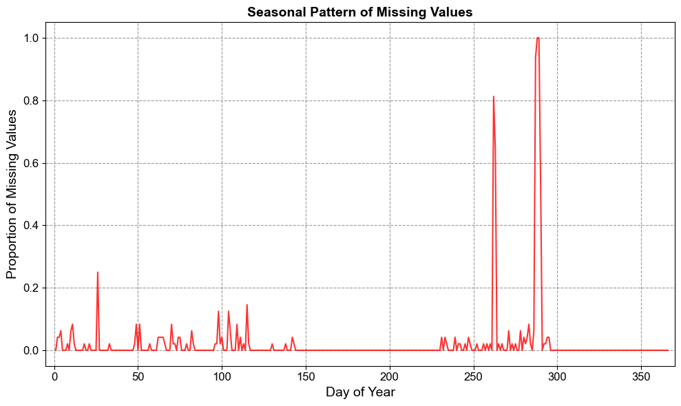
• Seasonal patterns may emerge if certain times of the year consistently show more missing data.

• This could be due to environmental factors (e.g., flooding or freezing affecting sensors).

2.2.4. Correlation Between Missingness and Recorded Values

To determine if there is a relationship between recorded values and missingness, we analyze whether low or high gage height (ft) readings are more likely to precede or follow gaps:

Show code cell source

Hide code cell source

df['gage height (ft)'] = pd.to_numeric(df['gage height (ft)'], errors='coerce')
# Lagged correlation between recorded values and subsequent missingness
df['lagged_missing'] = df['gage height (ft)'].isnull().shift(-1)
correlation = df['gage height (ft)'].corr(df['lagged_missing'])

print(f"Correlation between gage height and subsequent missingness: {correlation:.2f}")

Correlation between gage height and subsequent missingness: -0.04

Interpreting this result:

• The correlation is very close to zero, suggesting there’s practically no linear relationship between the gage height and whether the next measurement will be missing.

• The slight negative value (-0.01) might indicate a very weak tendency for higher gage heights to be followed by non-missing values, but this relationship is negligible given how close to zero the correlation is.

Remember that this correlation doesn’t imply causation, and given its near-zero value, it suggests that the gage height doesn’t have a meaningful impact on whether the subsequent measurement will be missing or not.

2.2.5. Little’s MCAR Test

Little’s MCAR test [Little, 1988] is a multivariate statistical test that evaluates whether the overall missing data pattern across an entire dataset is consistent with the MCAR assumption. Unlike univariate approaches, it provides a comprehensive assessment by examining all variables simultaneously.

Methodology

Little’s MCAR test operates through a sophisticated statistical framework:

• Expectation-Maximization (EM) Algorithm: Estimates population parameters (means, covariances) under the MCAR assumption

• Pattern-Based Analysis: Identifies all unique missing data patterns in the dataset

• Mean Comparison: Compares observed group means for each pattern with EM-estimated expected means

• Chi-Square Statistic: Calculates test statistic based on these mean differences across patterns

• Hypothesis Testing: Tests H₀: All missing data in the dataset is MCAR

2.2.5.1. Example: Weather Time Series Analysis

Consider a temperature monitoring dataset with missing readings and categorical weather conditions:

Show code cell source

Hide code cell source

import numpy as np
import pandas as pd

# Create a sample time series DataFrame
dates = pd.date_range(start='2024-01-01', periods=30, freq='D')
data_ts = pd.DataFrame({
    'Temperature': [22, 23, np.nan, 25, 24, np.nan, 26, 27, 28, 29, 30, np.nan,
                    21, 22, 23, 24, 25, 26, 27, np.nan, 28, 29, 30, 31, 32,
                    33, 34, np.nan, 35, 36],
    'Humidity': [70, 72, 75, 68, 70, 71, 73, 75, 76, 78, 79, 80,
                 65, 67, 69, 70, 71, 73, 74, 75, 76, 77, 78, 79, 80,
                 81, 82, 83, 84, 85],
    'Weather_Condition': ['Sunny', 'Sunny', 'Cloudy', 'Sunny', 'Cloudy', 'Rainy',
                          'Sunny', 'Cloudy', 'Sunny', 'Rainy', 'Sunny', 'Cloudy',
                          'Sunny', 'Sunny', 'Cloudy', 'Sunny', 'Cloudy', 'Rainy',
                          'Sunny', 'Cloudy', 'Sunny', 'Rainy', 'Sunny', 'Cloudy',
                          'Sunny', 'Rainy', 'Sunny', 'Cloudy', 'Sunny', 'Rainy']
}, index=dates)

# Introduce some missing values strategically to simulate non-MCAR
# Let's say temperature is more likely to be missing on 'Rainy' days (MNAR/MAR depending on Humidity)
data_ts.loc[data_ts['Weather_Condition'] == 'Rainy', 'Temperature'] = np.nan

# Ensure it's not perfectly correlated
data_ts.loc['2024-01-03', 'Temperature'] = np.nan # Introduce some random missingness
data_ts.loc['2024-01-12', 'Temperature'] = np.nan # Introduce some random missingness
data_ts.loc['2024-01-20', 'Temperature'] = np.nan # Introduce some random missingness
data_ts.loc['2024-01-28', 'Temperature'] = np.nan # Introduce some random missingness


print("Sample Time Series Data:")
display(data_ts)

Sample Time Series Data:

	Temperature	Humidity	Weather_Condition
2024-01-01	22.0	70	Sunny
2024-01-02	23.0	72	Sunny
2024-01-03	NaN	75	Cloudy
2024-01-04	25.0	68	Sunny
2024-01-05	24.0	70	Cloudy
2024-01-06	NaN	71	Rainy
2024-01-07	26.0	73	Sunny
2024-01-08	27.0	75	Cloudy
2024-01-09	28.0	76	Sunny
2024-01-10	NaN	78	Rainy
2024-01-11	30.0	79	Sunny
2024-01-12	NaN	80	Cloudy
2024-01-13	21.0	65	Sunny
2024-01-14	22.0	67	Sunny
2024-01-15	23.0	69	Cloudy
2024-01-16	24.0	70	Sunny
2024-01-17	25.0	71	Cloudy
2024-01-18	NaN	73	Rainy
2024-01-19	27.0	74	Sunny
2024-01-20	NaN	75	Cloudy
2024-01-21	28.0	76	Sunny
2024-01-22	NaN	77	Rainy
2024-01-23	30.0	78	Sunny
2024-01-24	31.0	79	Cloudy
2024-01-25	32.0	80	Sunny
2024-01-26	NaN	81	Rainy
2024-01-27	34.0	82	Sunny
2024-01-28	NaN	83	Cloudy
2024-01-29	35.0	84	Sunny
2024-01-30	NaN	85	Rainy

Utilizing MCARTest from [Schouten et al., 2022]:

Show code cell source

Hide code cell source

from pyampute.exploration.mcar_statistical_tests import MCARTest
from sklearn.preprocessing import LabelEncoder

data_ts_num = data_ts.copy()

le = LabelEncoder()
data_ts_num['Weather_Condition'] = le.fit_transform(data_ts_num['Weather_Condition'])

# Perform Little's MCAR test
mt = MCARTest(method="little")
p_value = mt.little_mcar_test(data_ts_num)

print(f"Little's MCAR test p-value: {p_value:.4f}")

# Interpretation
if p_value < 0.05:
    print("Reject H₀: Strong evidence that data is NOT MCAR")
else:
    print("Fail to reject H₀: Data is consistent with MCAR assumption")

Little's MCAR test p-value: 0.0000
Reject H₀: Strong evidence that data is NOT MCAR

A p-value of 0.0000 from Little’s MCAR test provides clear statistical evidence that the missing data in the dataset is not completely at random. This means that the pattern of missing values—in this case, temperature readings—is systematically related to other observed factors rather than occurring randomly throughout the dataset.

2.2.6. Chi-Square Test for MCAR Assessment in Time Series Data

While Little’s MCAR test [Li, 2013, Little, 1988] remains the standard for comprehensive multivariate assessment of missing data patterns, the Chi-square test provides a focused approach to examine the relationship between missingness in a specific time series variable and categorical or time-based features. This method is particularly valuable for preliminary assessments and understanding localized missingness patterns.

Test Setup and Procedure

1. Create Missingness Indicator
Generate a binary variable (e.g., Variable_missing) where:

• 1 = missing value in the target time series variable

• 0 = observed value

2. Select Comparative Variable
Choose an appropriate categorical or derived time-based feature from your dataset, such as:

• Day of week

• Month or season

• Weather conditions

• Equipment status categories

3. Construct Contingency Table
Create a cross-classification table showing the frequency distribution of observed versus missing values across categories of the comparative variable.

4. Execute Chi-Square Test of Independence
Apply the test with the following hypotheses:

• H₀ (Null): Missingness is independent of the comparative variable (consistent with MCAR)

• H₁ (Alternative): Missingness depends on the comparative variable (suggests non-MCAR)

5. Statistical Interpretation

• p-value < α (typically 0.05): Reject H₀. Strong evidence that missingness is related to the comparative variable, indicating the data is likely not MCAR

• p-value ≥ α: Fail to reject H₀. Insufficient evidence of dependency, consistent with MCAR for this specific relationship

Implementation:

Show code cell source

Hide code cell source

import pandas as pd
import numpy as np
from scipy.stats import chi2_contingency


def chi_square_mcar_test_ts(data, variable_with_missing, other_variable):
    """
    Performs a Chi-square test to assess if missingness in a time series variable
    is related to another categorical or time-based feature.

    Parameters
    ----------
    data : pd.DataFrame
        Input DataFrame, ideally with a datetime index
    variable_with_missing : str
        Name of the time series variable with missing values to test
    other_variable : str
        Name of categorical variable or derived time feature (e.g., 'DayOfWeek')
        to compare against missingness patterns

    Returns
    -------
    tuple
        - chi2 (float): Chi-square test statistic
        - p_value (float): P-value of the test
        - conclusion (str): Interpretation of MCAR hypothesis test results
    """
    data_copy = data.copy()
    data_copy[f'{variable_with_missing}_missing'] = (
        data_copy[variable_with_missing].isnull().astype(int)
    )

    # Create contingency table
    contingency_table = pd.crosstab(
        data_copy[f'{variable_with_missing}_missing'],
        data_copy[other_variable]
    )

    # Perform Chi-square test of independence
    chi2, p_value, _, _ = chi2_contingency(contingency_table)

    # Interpret results
    alpha = 0.05
    if p_value < alpha:
        conclusion = (
            f"Reject the null hypothesis: Missingness in '{variable_with_missing}' "
            f"is likely not MCAR in relation to '{other_variable}' (p-value={p_value:.4f})."
        )
    else:
        conclusion = (
            f"Do not reject the null hypothesis: Missingness in '{variable_with_missing}' "
            f"is potentially MCAR in relation to '{other_variable}' (p-value={p_value:.4f})."
        )

    return chi2, p_value, conclusion

Continuing with our weather data example:

Show code cell source

Hide code cell source

# Perform MCAR tests
print("=== MCAR Testing Results ===")

# Test 1: Temperature vs Weather Condition
chi2_weather, p_weather, conclusion_weather = chi_square_mcar_test_ts(
    data_ts, 'Temperature', 'Weather_Condition'
)
print(f"Temperature vs. Weather Condition:")
print(f"Chi-square: {chi2_weather:.4f}, p-value: {p_weather:.4f}")
print(conclusion_weather)

print("\n" + "-"*50)

# Test 2: Temperature vs Day of Week
data_ts['DayOfWeek'] = data_ts.index.day_name()
chi2_dow, p_dow, conclusion_dow = chi_square_mcar_test_ts(
    data_ts, 'Temperature', 'DayOfWeek'
)
print(f"Temperature vs. Day of Week:")
print(f"Chi-square: {chi2_dow:.4f}, p-value: {p_dow:.4f}")
print(conclusion_dow)

=== MCAR Testing Results ===
Temperature vs. Weather Condition:
Chi-square: 20.0000, p-value: 0.0000
Reject the null hypothesis: Missingness in 'Temperature' is likely not MCAR in relation to 'Weather_Condition' (p-value=0.0000).

--------------------------------------------------
Temperature vs. Day of Week:
Chi-square: 2.5500, p-value: 0.8628
Do not reject the null hypothesis: Missingness in 'Temperature' is potentially MCAR in relation to 'DayOfWeek' (p-value=0.8628).

For our actual dataset, the Chi-square test for “Temperature vs. Weather Condition” yields a statistic of 20.0000 and a p-value of 0.0000, providing overwhelming evidence that missing temperature values are not randomly distributed across weather types. In our data, nearly every “Rainy” day is linked to a missing temperature, while “Sunny” days almost always have recorded temperatures, and “Cloudy” days are a mix but tend to have more observed values.

This clear pattern points to a strong relationship between adverse weather and missing temperature measurements. The missingness may stem from equipment malfunction during rain, intentional omission of data in challenging conditions, or other process issues associated with rainfall. A p-value this low means the connection between rain and missing temperatures is so pronounced that it cannot be attributed to random variation alone. In other words, on “Rainy” days, the likelihood of missing temperature records is exceptionally high, confirming that our data are not missing completely at random.

By contrast, for “Temperature vs. Day of Week,” the much higher p-value (0.8628) shows that missing temperature readings do not cluster on any particular day of the week. This lack of association indicates that, in our data, the time of the week does not influence whether a temperature is recorded or missing, so missingness is—by this measure—consistent with MCAR. This distinction demonstrates that while weather explains the missingness pattern, the day of the week does not in our dataset.

Your write-up is solid and provides clear, actionable information about the risks of simple methods and the advantages/limitations of advanced imputation strategies when MCAR is rejected. Here’s a revised, more concise version for greater clarity and flow, while retaining your key points and adding slight polish:

---

2.2.6.1. When MCAR Is Rejected (Non-Random Missingness)

Risk Assessment:

• Listwise deletion can introduce systematic bias by disproportionately removing certain observations, leading to incorrect conclusions about the underlying process.

• Simple imputation methods (such as mean or median) ignore the reason for missingness, typically underestimate variance, and can distort variable relationships.

• Results may be skewed toward specific conditions or time periods, resulting in inaccurate parameter estimates and potentially misleading findings.

Table 2.1 Recommended Treatment Strategies

Method	When to Use	Advantages	Considerations
Multiple Imputation	General use; assumes MAR	Handles uncertainty in missing values, accurate estimates	Computationally intensive; requires MAR, model spec
Regression Imputation	Predictors available; assumes MAR	Leverages observed relationships	May underestimate variability; assumes linearity
Time Series Imputation	Presence of temporal dependencies	Utilizes sequence structure, well-suited for time series	Each method has specific assumptions
ARIMA-based Imputation	Complex trends or seasonality	Captures autocorrelation, trend, seasonality	Requires correct model specification (p, d, q)
Machine Learning Imputation	Complex, nonlinear patterns	Handles sophisticated relationships; can improve accuracy	Risk of overfitting; needs careful validation

Note: Overfitting—when an imputation model fits the idiosyncrasies of the training data but fails to generalize—should be guarded against, especially with machine learning methods.