Remark
Please be aware that these lecture notes are accessible online in an ‘early access’ format. They are actively being developed, and certain sections will be further enriched to provide a comprehensive understanding of the subject matter.
1.6. Cross-Correlation in Time Series#
In this section, we explore Cross-Correlation, a metric used to measure the similarity between two time series as a function of the time displacement (lag) between them. This is a fundamental tool in geophysical and environmental data science for identifying “lead-lag” relationships—determining if one signal (e.g., temperature in Calgary) has a predictive relationship with another (e.g., temperature in Columbia).
1.6.1. Mathematical Background#
To understand how two signals relate, we look at them in both the Time Domain (looking at time delays) and the Frequency Domain (looking at cycles).
1.6.1.1. Time Domain Definition#
Mathematically, the relationship starts with the “sliding dot product” known as the cross-covariance. For two sequences \(x_t\) and \(y_t\) at lag \(\tau\), this is:
However, the magnitude of this sum depends on the units of the data. To make the metric comparable across different datasets, we normalize it by the standard deviations. This yields the Sample Cross-Correlation Function (CCF), denoted as \(\hat{\rho}_{xy}(\tau)\) [Brockwell and Davis, 2016]:
Where:
\(\mu_x, \mu_y\): Means of the series.
\(\sigma_x, \sigma_y\): Standard deviations of the series.
\(\tau\): The lag (shift) in time steps.
\(N\): The number of observations.
Interpretation: The resulting value ranges from \(-1\) to \(+1\):
Peak at \(\tau = 0\): The series are synchronized.
Peak at \(\tau > 0\): \(x_t\) leads \(y_t\) (Current \(x\) predicts future \(y\)).
Peak at \(\tau < 0\): \(y_t\) leads \(x_t\) (Future \(x\) predicts current \(y\), or \(x\) lags \(y\)).
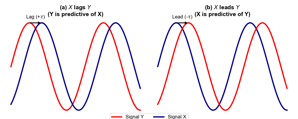
Fig. 1.11 Lead–lag concept for cross-correlation. Red curve is signal \(Y\) and blue curve is signal \(X\). Panel (a) shows a positive time shift where \(X\) occurs later than \(Y\) (\(X\) lags \(Y\)), so \(Y\) is predictive of future \(X\); panel (b) shows a negative shift where \(X\) occurs earlier than \(Y\) (\(X\) leads \(Y\)), so \(X\) is predictive of future \(Y\). Note that the sign of “lag” depends on the cross-correlation definition and software convention; here using scipy.signal.correlate(target, source), a positive optimal lag means the source series leads the target and must be shifted forward by that many time steps to align visually.#
1.6.1.2. Frequency Domain: Concepts#
While cross-correlation gives one “best” lag, it effectively averages over all time scales in the data (day-to-day swings and slow seasonal cycles mixed together). Frequency-domain thinking helps answer: “Are these two series related mainly through seasons (slow cycles), synoptic weather (multi-day cycles), or fast local noise?”
Frequency (\(f\)) vs. Period (\(T\))
A cycle can be described in two equivalent ways:
Period (\(T\)): Time for one full repeat (e.g., 365 days).
Frequency (\(f\)): Repeats per unit time (e.g., cycles/day).
They are inverses:
Examples (daily data):
Annual cycle: \(T = 365\) days \(\Rightarrow f \approx 1/365 \approx 0.0027\) cycles/day.
Weekly / synoptic: \(T = 7\) days \(\Rightarrow f \approx 1/7 \approx 0.143\) cycles/day.
Notes (units + sampling)
Units must match (dimensional check).
The identity \(f = 1/T\) is always true, but the time unit you use for \(T\) determines the unit of \(f\):If \(T\) is in seconds, \(f\) is cycles/second = Hertz (Hz).
If \(T\) is in days, \(f\) is cycles/day.
A quick sanity check: if you say “a 7‑day cycle,” the frequency must be “about 0.14 cycles/day,” not Hz.
Sampling frequency is how the code knows your time unit.
For evenly sampled data, define the sampling interval \(\Delta t\) and sampling frequency \(f_s\):\(\Delta t\) = time between observations (e.g., 1 day).
\(f_s = 1/\Delta t\) (e.g., \(f_s = 1\) sample/day).
In many Python signal-processing functions, if you do not provide \(f_s\), the frequency axis may be returned in “cycles per sample” rather than “cycles per day,” which makes it easy to misread where the annual or weekly peaks should appear.
1.6.1.3. Frequency Domain: Coherence#
While cross-correlation measures similarity in the time domain, Coherence measures the correlation between two signals as a function of frequency. It is analogous to a squared correlation coefficient for each frequency component.
The Magnitude Squared Coherence \(C_{xy}(f)\) is defined as:
Where:
\(P_{xy}(f)\): Cross-spectral density between \(x\) and \(y\).
\(P_{xx}(f), P_{yy}(f)\): Power spectral densities of \(x\) and \(y\) respectively.
Values of \(C_{xy}(f)\) near 1 indicate a strong linear relationship at that frequency, while values near 0 indicate no relationship.
This efficiency is why standard libraries (such as scipy.signal.correlate) often use FFT-based methods (method='fft') for larger arrays.
1.6.2. Example: Columbia vs. Calgary Temperatures#
To illustrate cross-correlation and coherence, we analyze daily mean temperatures from Columbia, Missouri (target, at 92°W) and Calgary, Alberta (source, at 114°W) during 2024. These cities are separated by over 2,000 km with distinct climates: Calgary is colder year-round due to higher latitude and continental exposure, while Columbia experiences milder winters and more humid summers. The data spans is sourced from https://open-meteo.com/ with daily temperatures means measured in degrees Celsius.
The key scientific question is: Do weather systems that affect Calgary (west) influence Columbia (east) with a detectable time delay? North American weather systems typically propagate eastward, so we hypothesize that Calgary’s temperature anomalies (unusually warm or cold days) may “lead” Columbia’s by a few days. Cross-correlation will quantify this lead-lag timing, and coherence will tell us whether this relationship is strongest at the seasonal scale, the synoptic (3–7 day) scale, or both.
We will apply this theory to analyze the relationship between daily temperatures in Columbia, MO, and Calgary, AB for the year 2024. Given the prevailing West-to-East weather patterns in North America, we hypothesize that temperature changes in Calgary (West) might “lead” similar changes in Columbia (East).
1.6.2.1. Visualizing and Comparing the Series#
We will analyze the daily mean temperatures of Calgary, AB and Columbia, MO for the year 2024. Note that Calgary (approx. 114°W) is significantly west of Columbia (approx. 92°W). Since weather systems in North America often move West-to-East, we might hypothesize a lag relationship.
Before diving into mathematical metrics, it is essential to visually inspect the time series. Here, we compare the daily mean temperatures of Calgary, Canada, and Columbia, Missouri.
Although these two cities are geographically distinct—separated by over 2,000 km and different climate zones—they are both located in the Northern Hemisphere. Therefore, we expect them to share a strong seasonal component (the annual temperature cycle).
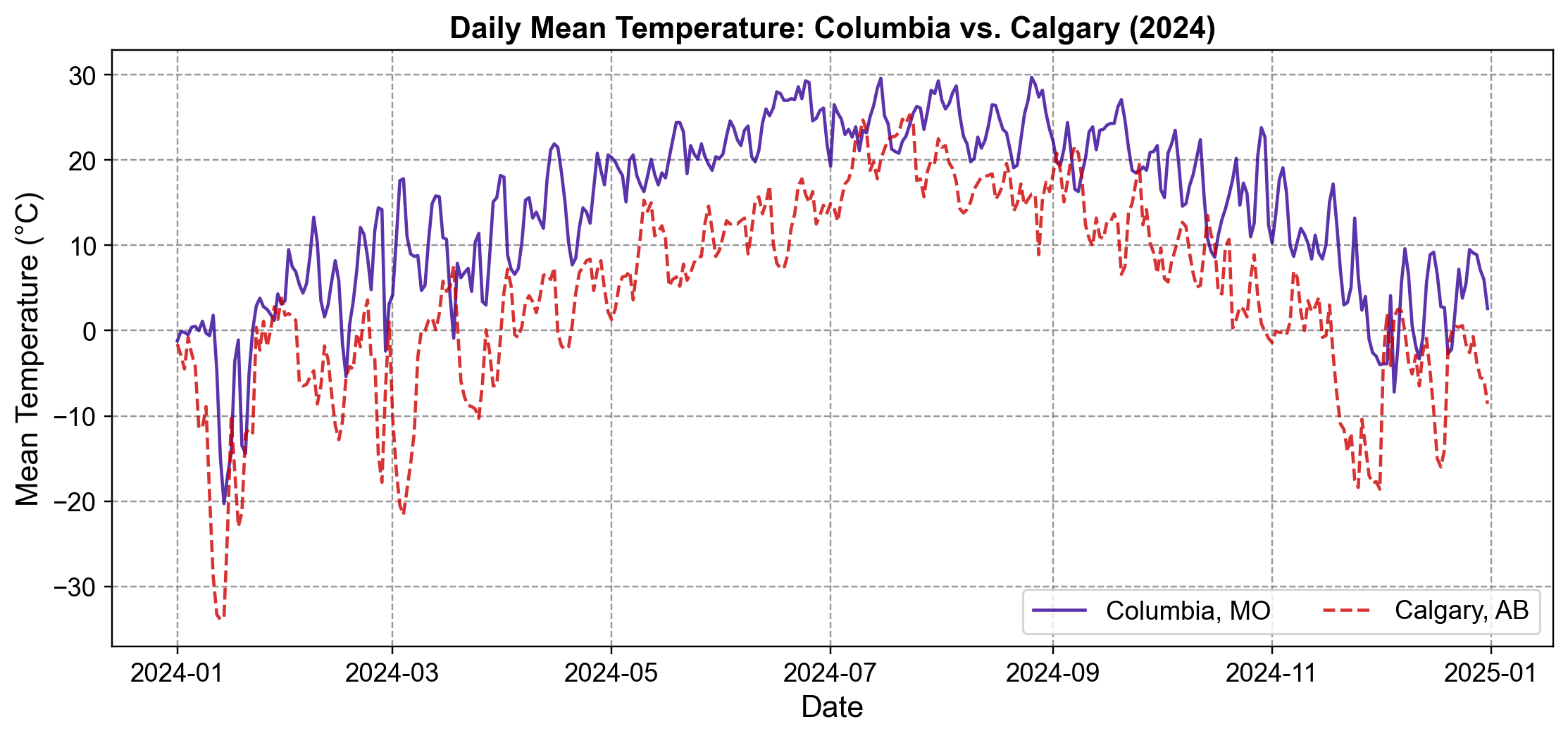
Fig. 1.12 Daily mean temperature in Columbia, MO (solid, purple) and Calgary, AB (dashed, red) for 2024. The series share a clear annual seasonal cycle (warming in summer, cooling in winter), but differ in amplitude and baseline. Notably, many warm and cold spells appear to occur nearly simultaneously, though slight timing offsets may exist within short intervals. This visual similarity motivates the search for an optimal time lag.#
Visual observations:
Both series follow a sinusoidal annual rhythm: winter minima (January, December) and summer maxima (July, August) occur at nearly the same calendar dates.
Amplitude asymmetry: Calgary’s curve swings from roughly −30°C to +20°C, while Columbia ranges from −20°C to +30°C. This reflects Calgary’s continental climate (larger extremes) versus Columbia’s more temperate profile.
Apparent synchrony: Many rapid warm-ups and cold snaps seem to happen together (e.g., both cities warm in April, cool in September), suggesting shared synoptic weather drivers.
This visual alignment is reassuring—it tells us the two locations are not independent—but it doesn’t yet answer: Is there a small time delay? And which timescale (seasonal vs. weekly) matters most?
1.6.2.2. Time‑Domain Analysis – When Does One Series Lead the Other?#
To answer “When?”, we compute the normalized cross-correlation function (CCF) across a range of lags. Recall the normalized CCF (from (1.3))
Interpretation logic:
If the CCF peaks at \(\tau = +2\), this means: shift Calgary forward by 2 days, and the two series match best. In meteorological terms, Calgary’s temperature anomalies arrive 2 days before Columbia’s. Put plainly: a cold spell in Calgary on January 10 tends to reach Columbia around January 12.
If the peak were at \(\tau = -2\), it would mean Columbia leads Calgary—physically implausible for eastward-moving systems.
A peak near \(\tau = 0\) would mean the cities respond simultaneously to the same large-scale weather driver (e.g., the seasonal cycle), without a propagation delay.
Next, we move from what the series look like to when one location tends to follow the other by examining the cross‑correlation and a lagged overlay of the two series. We visualize the results to confirm the relationship. A negative lag implies the “Source” (Calgary) leads the “Target” (Columbia).
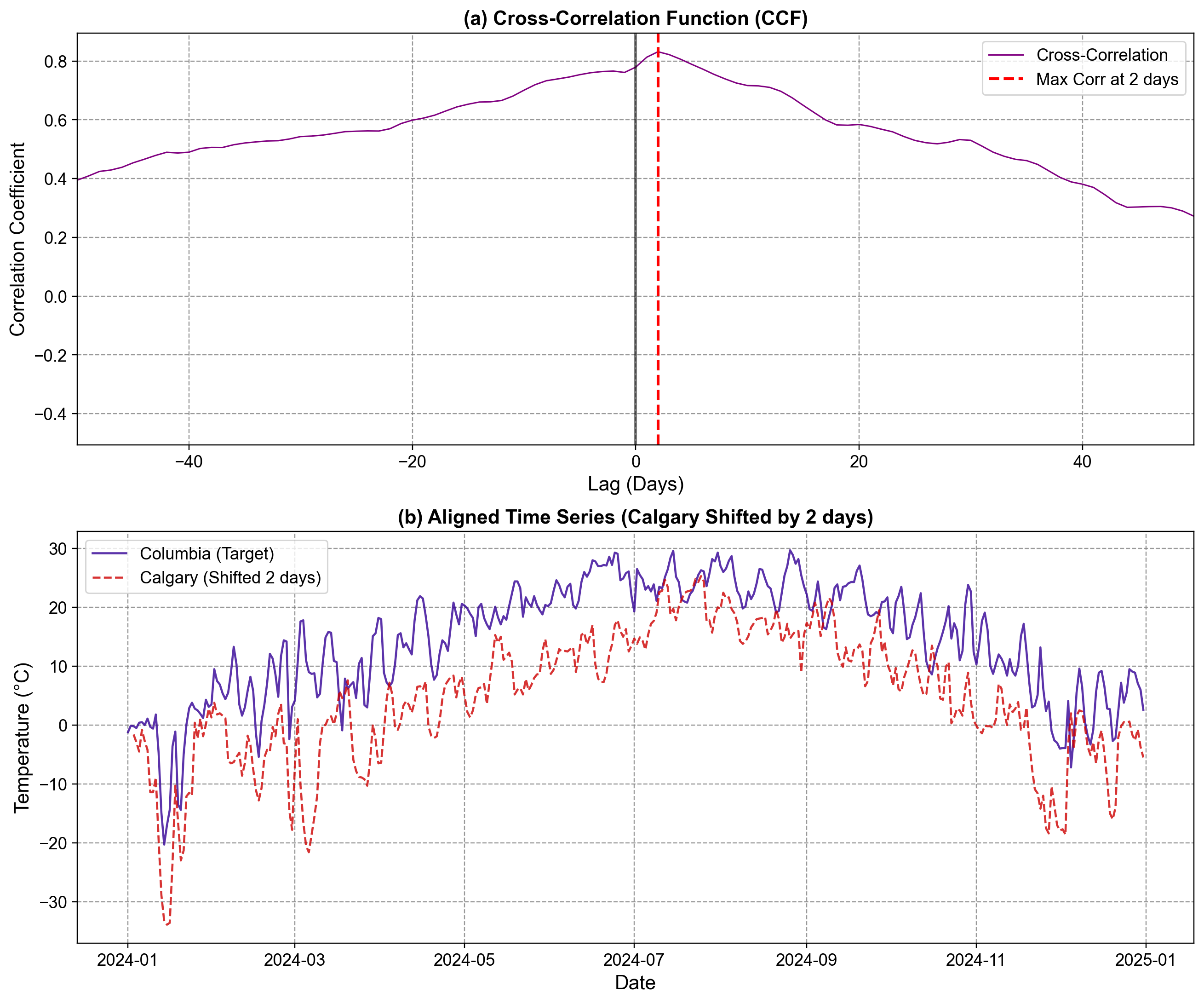
Fig. 1.13 (a) Normalized cross-correlation between Calgary and Columbia daily temperatures for lags from −50 to +50 days. The peak occurs at \(\tau = +2\) days with a correlation of 0.83, substantially higher than the lag-0 correlation of 0.78. The dashed red line marks the optimal lag; the vertical black line shows lag zero for reference. (b) Time series overlay after shifting Calgary by +2 days. The two curves now track closely, confirming visual alignment. Deviations reflect either local weather noise or synoptic features that do not propagate uniformly across the distance.#
Interpretation:
The 2-day lead makes meteorological sense. Weather systems (cold fronts, high-pressure ridges) that originate in the Pacific or Rocky Mountain region reach Calgary first, then propagate eastward at a typical speed of ~1,000 km per 2 days, arriving at Columbia 2–3 days later. This is consistent with observed wind speeds in the troposphere (~30–40 m/s at jet stream altitudes) and surface pressure perturbation propagation.
The correlation magnitude (0.83) is high but not perfect (1.0). Why? Because:
Local effects (urban heat island, local orography) introduce noise at each location.
Some weather systems weaken or split during eastward travel.
The 2-day lag is an average; some events lead by 1 day, others by 3, creating scatter.
Note
Lag answers the question: “How many days early does Location A predict Location B’s anomalies?” A positive lag means the source (Calgary) is predictive of the future target (Columbia); we are not claiming causality, only that they share a time-shifted correlation structure consistent with eastward weather propagation.
1.6.2.3. Frequency‑Domain Analysis – At What Time‑Scales Are the Cities Linked?#
We have established that Calgary generally leads Columbia by 2 days. Now we ask a deeper question: “Does this link exist for all weather patterns, or only specific ones?”
To answer this, we move from the Time Domain (Lead/Lag) to the Frequency Domain (Cycles).
Conceptual setup:
Imagine decomposing each time series into “layers” at different frequencies. We look for correlation in specific bands:
Low Frequency: Annual seasonality (\(T \approx 365\) days).
Intermediate Frequency: Synoptic weather systems (\(T \approx 3-7\) days).
High Frequency: Local noise (\(T < 3\) days).
Recall our unit conversion:
Annual: \(f \approx 1/365 \approx 0.0027\) cycles/day.
Weekly: \(f \approx 1/7 \approx 0.143\) cycles/day.
We will use Coherence to measure the strength of the relationship (0 to 1) at each frequency.
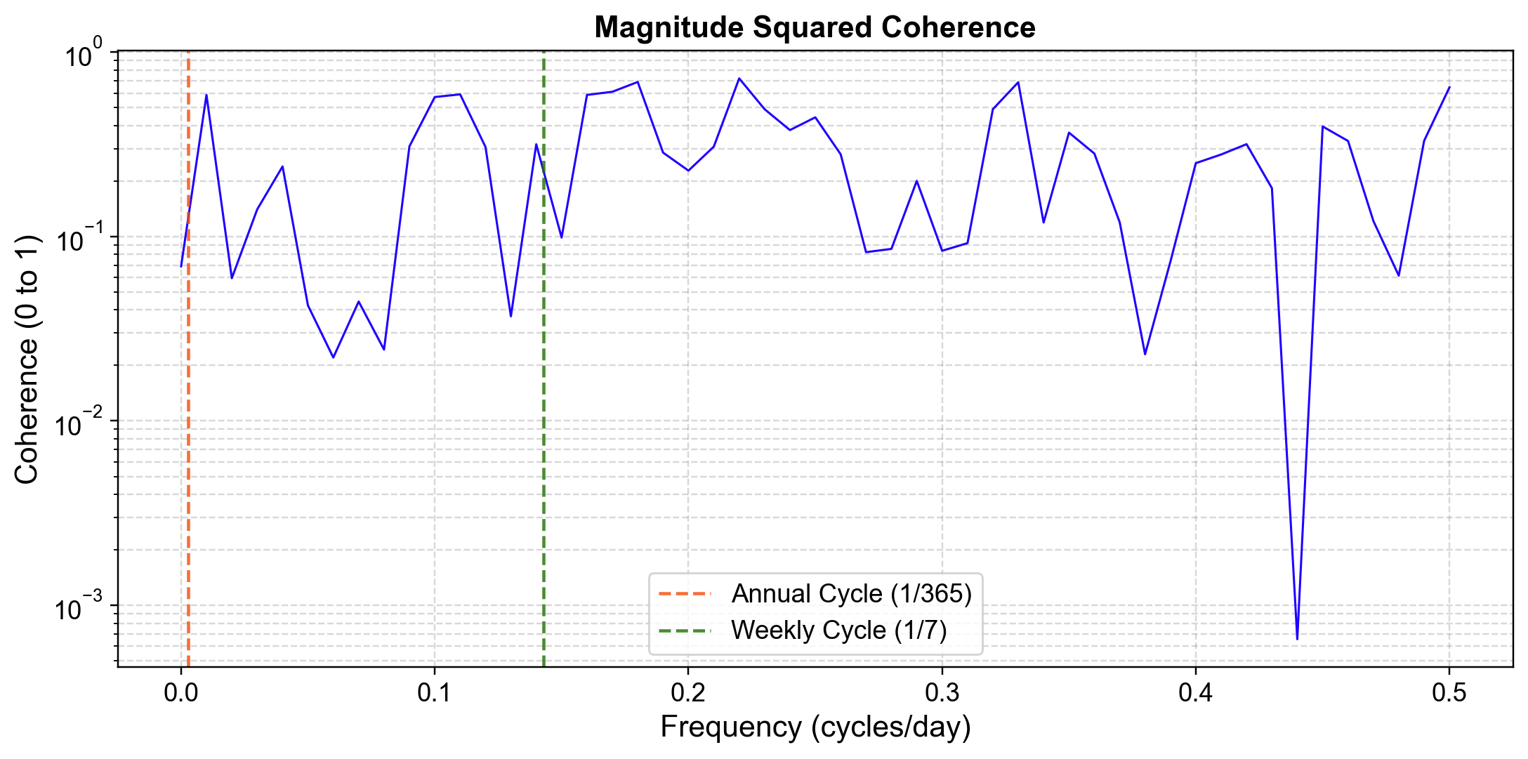
Fig. 1.14 Magnitude-squared coherence between Calgary and Columbia daily temperatures versus frequency (in cycles per day). Two vertical dashed lines mark reference timescales: the annual cycle at 1/365 ≈ 0.0027 cycles/day (red), and the weekly cycle at 1/7 ≈ 0.143 cycles/day (green). Coherence peaks sharply near the annual frequency (as expected), but importantly remains high in the 3–7 day band (around 0.15 cycles/day), indicating that synoptic weather patterns drive a substantial portion of the shared variability beyond simple seasonality.#
Interpretation:
Low Frequencies (Left side, Annual):
Coherence \(\approx\) 1.0.
Physics: This is the seasonal envelope. Both cities warm up in summer and cool down in winter. This is expected (trivial), but confirms the data quality.
Intermediate Frequencies (The “Synoptic Band”, Center):
Coherence \(\approx\) 0.4 – 0.6.
Physics: This is the critical finding. Look at the top axis between “Week” and “3 Days” (\(f \approx 0.14\)). The coherence is well above zero. This proves that Synoptic Weather Systems (cold fronts, high pressure ridges) are a shared driver. The same storm system that hits Calgary propagates to Columbia.
High Frequencies (Right side, < 3 Days):
Coherence drops.
Physics: Brief, local events—like afternoon thunderstorms or local wind shifts—are independent. A random storm in Calgary does not predict a random storm in Columbia 2 days later.
At what frequencies do the cities behave like a single system?
They are coupled at the Annual scale (Seasons) and the Synoptic scale (Weather Patterns), but decoupled at the Local scale (Noise).
1.6.2.4. Synthesis: Lag and Coherence#
The cross‑correlation and coherence results answer complementary questions in a compact way:
Aspect |
Question |
Answer from Data |
|---|---|---|
Timing (Time Domain) |
How many days does Calgary lead Columbia? |
≈2 days (CCF peak at \(\tau = +2\)) |
Correlation strength (Time Domain) |
How strong is the link at that lag? |
\(r \approx 0.83\) (higher than lag 0) |
Seasonal linkage (Frequency Domain) |
Are annual cycles shared? |
Yes, coherence ≈ 1 at 1/365 cycles/day |
Synoptic linkage (Frequency Domain) |
Are 3–7 day systems shared? |
Yes, coherence stays elevated near 1/7 cycles/day |
Local variability (Frequency Domain) |
Are sub‑3‑day fluctuations shared? |
Mostly no, coherence drops at high frequencies |
Notes
Why do we need both analyses?
Cross-correlation reveals when one location predicts another (the 2-day lead); coherence reveals which timescales matter (synoptic systems dominate, not just annual seasonality). Together, they expose the mechanisms linking the two cities: large-scale weather systems propagating eastward at ~1,000 km/2 days, while local boundary-layer processes remain independent.Note on Practical Use: In operations, knowing that Calgary temperature anomalies lead Columbia by ~2 days allows meteorologists to use Calgary observations to improve short-range forecasts for Columbia. However, the imperfect correlation (0.83, not 1.0) reflects real variability in propagation speed and system intensity—a useful reminder that statistical relationships never replace physical reasoning.