Remark
Please be aware that these lecture notes are accessible online in an ‘early access’ format. They are actively being developed, and certain sections will be further enriched to provide a comprehensive understanding of the subject matter.
3.3. Additive vs. Multiplicative Decomposition#
3.3.1. Mathematical Framework#
For a time series \(y_t\), two decomposition models exist [Cleveland et al., 1990, Wen et al., 2019, Wen et al., 2020]:
Additive model (appropriate when seasonal amplitude is constant):
Multiplicative model (appropriate when seasonal amplitude grows with trend):
When seasonal variations scale proportionally with the series level, a multiplicative model is more appropriate. STL, which assumes an additive structure, handles multiplicative data via logarithmic transformation:
After decomposing \(\log(y_t)\) additively, components are back-transformed:
where \(\tilde{T}_t\), \(\tilde{S}_t\), \(\tilde{R}_t\) are the additive components of \(\log(y_t)\).
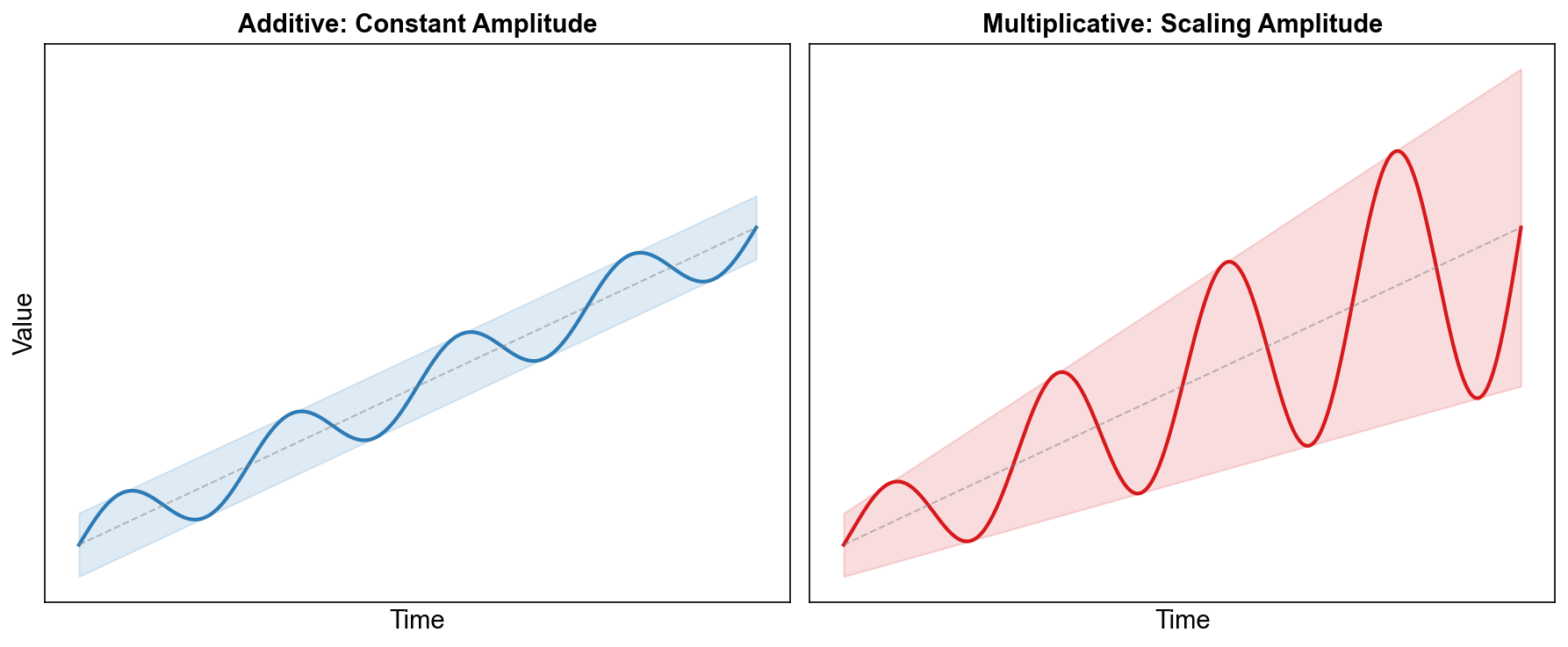
Fig. 3.13 Stylized illustration of additive versus multiplicative seasonality. Left panel: Additive model with constant seasonal amplitude (the vertical distance between peaks and troughs is fixed at ±4 units, regardless of the trend level). Right panel: Multiplicative model where seasonal amplitude scales with the level of the trend (the band is ±40% of the local trend), so seasonal swings become larger in absolute terms as the series grows, while remaining comparable in relative percentage terms.#
3.3.2. Example: Air Passengers (Multiplicative Decomposition)#
The classic Air Passengers dataset (monthly totals from 1949–1960) exhibits clear multiplicative seasonality: seasonal fluctuations grow proportionally with the increasing trend in air travel demand.
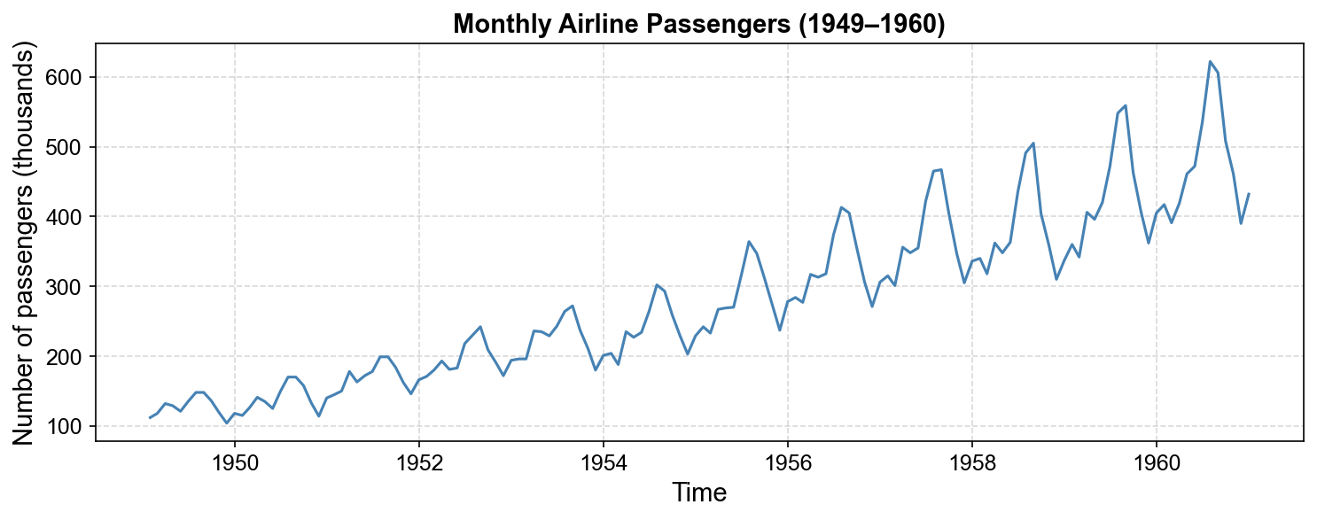
Fig. 3.14 Monthly airline passenger totals from January 1949 to December 1960. The series exhibits a strong upward trend with clear seasonal peaks during summer months (June–August). Crucially, the amplitude of seasonal fluctuations increases proportionally with the trend level, indicating multiplicative rather than additive seasonality.#
3.3.3. Additive vs. Multiplicative: Visual Comparison#
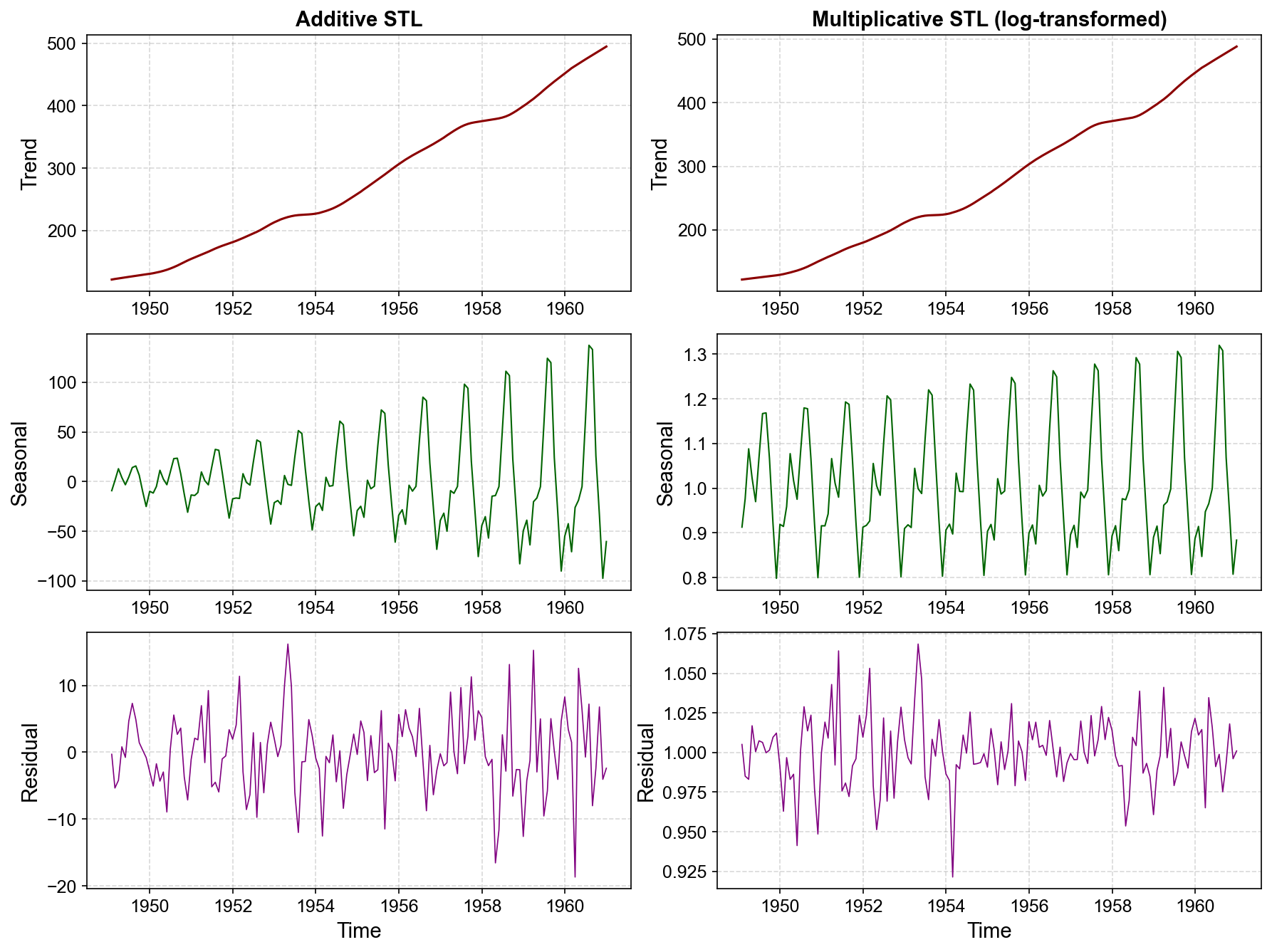
Fig. 3.15 Comparison of additive (left) versus multiplicative (right) STL decomposition for the Air Passengers series. Left panels: Additive decomposition incorrectly assumes constant seasonal amplitude, leading to increasing residual variance over time as the model fails to account for growing seasonal fluctuations. Right panels: Multiplicative decomposition (via log-transformation) correctly captures proportional seasonal growth, yielding residuals with stable variance throughout the series. The multiplicative model is appropriate for this dataset.#
Key Observations from Fig. 3.15
Trend: Captures overall growth but underestimates the acceleration.
Seasonal: Fixed amplitude (~20–30 passengers) throughout, failing to account for larger seasonal swings in later years.
Residual: Shows heteroscedasticity (increasing variance over time), indicating model misspecification.
Trend: Smooth exponential growth trajectory.
Seasonal: Amplitude proportional to trend level (e.g., seasonal multiplier ranges from 0.85 to 1.15, meaning ±15% variation around trend).
Residual: Homoscedastic (constant variance), confirming appropriate model choice.
3.3.4. Multiplicative Seasonal Pattern Example#
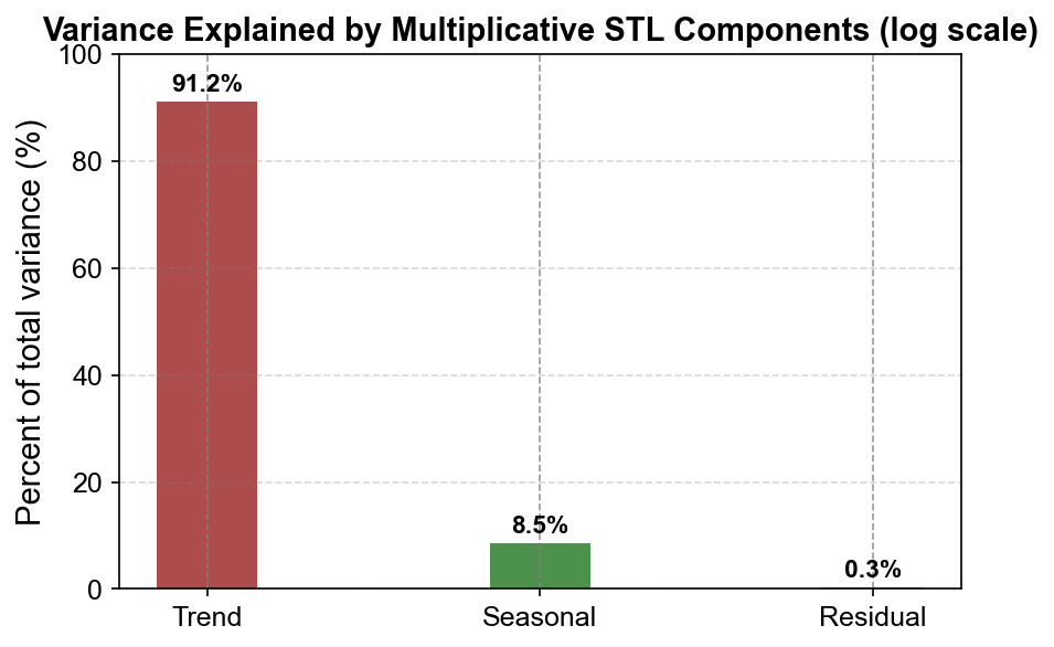
Fig. 3.16 Variance decomposition for the multiplicative STL decomposition of Air Passengers. The trend dominates, explaining approximately 91.15% of total log-variance, while seasonality accounts for ~8.53%, and residuals capture only ~0.25%, indicating an excellent fit.#
Component |
Variance (log scale) |
Percent_of_total |
|---|---|---|
Trend |
0.1776 |
91.1518 |
Seasonal |
0.0166 |
8.5292 |
Residual |
0.0005 |
0.2507 |
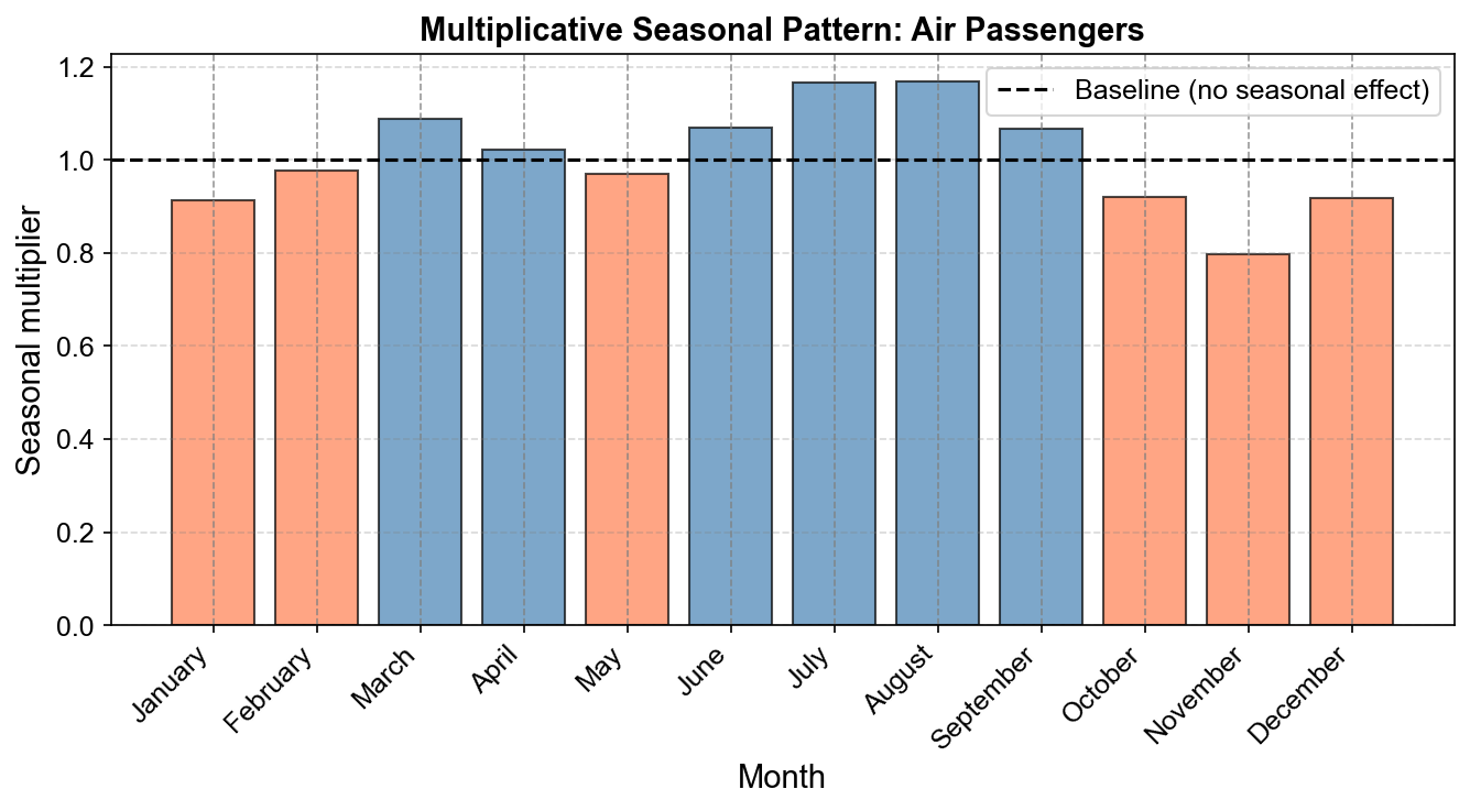
Fig. 3.17 Multiplicative seasonal pattern for Air Passengers (1949–1960). Each bar represents the seasonal multiplier for that month (e.g., July ≈ 1.13 means +13% above trend). Summer months (June–August) show strong positive seasonality (blue bars), while winter months (November–February) show negative seasonality (orange bars), reflecting vacation travel patterns.#
Month |
Seasonal_Multiplier |
Percent_Change |
|---|---|---|
January |
0.9128 |
-8.7185 |
February |
0.976 |
-2.4028 |
March |
1.0882 |
8.818 |
April |
1.0227 |
2.268 |
May |
0.9699 |
-3.0139 |
June |
1.0691 |
6.9107 |
July |
1.1671 |
16.7145 |
August |
1.1686 |
16.858 |
September |
1.0663 |
6.6333 |
October |
0.9206 |
-7.9434 |
November |
0.7982 |
-20.1813 |
December |
0.9189 |
-8.1087 |
Exponential trend growth: Air travel still exhibits strong exponential growth over 1949–1960, with passenger volumes increasing several‑fold over the sample, consistent with post‑war economic expansion and rapid adoption of commercial aviation.
Proportional seasonality: Seasonal multipliers now range from about 0.80 in November (roughly 20% below trend) to about 1.17 in July–August (roughly 17% above trend). This confirms a strongly multiplicative seasonal structure: as the baseline travel volume rises over time, the absolute seasonal swings become larger (e.g., from tens of thousands of passengers early in the sample to many tens of thousands later), while the relative percentage variation by month remains roughly stable from year to year.
Stable residuals: After accounting for the exponential trend and these proportional seasonal effects, the remaining residuals continue to show approximately constant variance and no systematic temporal pattern, indicating that the multiplicative decomposition captures the main systematic features of the series.
3.3.5. Reconstruction: Verifying the Multiplicative Decomposition#
Mean absolute reconstruction error: 0.0000
Root mean squared error: 0.0000
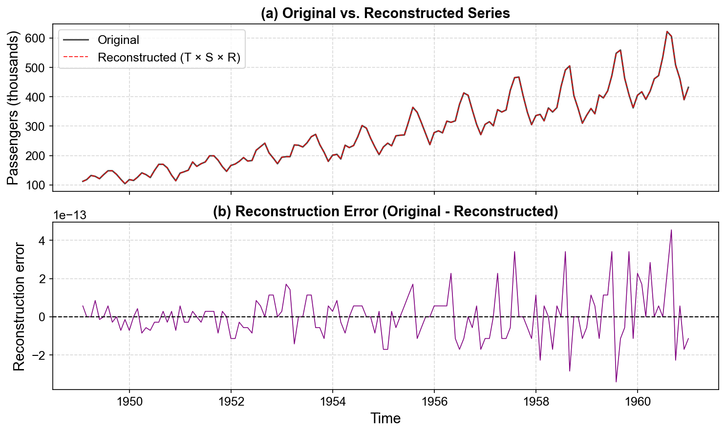
Fig. 3.18 Top panel: Original Air Passengers series (black) versus reconstructed series from multiplicative STL components \(T_t \times S_t \times R_t\) (red dashed). The two curves are nearly indistinguishable. Bottom panel: Reconstruction error, showing negligible deviations (< 1 passenger on average), confirming that the multiplicative decomposition accurately represents the observed data.#
3.3.6. Forecasting Implications#
For forecasting, the multiplicative decomposition enables:
where:
\(\hat{T}_{T+h}\) is an extrapolated trend (e.g., via exponential smoothing or regression on log-trend)
\(\hat{S}_{(T+h \mod 12)}\) is the seasonal multiplier for month \(h\)
This formulation ensures that forecasted seasonal fluctuations grow proportionally with the trend, unlike additive forecasts which would underestimate future seasonal peaks.
3.3.6.1. Example: STL-Based Multiplicative Forecasts#
Here, we construct a simple STL-based multiplicative forecast using the Air Passengers series:
Work on the log scale and reuse the multiplicative STL decomposition
stl_multiplicativealready computed earlier.Fit a linear trend to the STL trend component on the log scale.
Extrapolate the log-trend \(h\) steps ahead.
Reuse the seasonal pattern in a seasonal-naive fashion (cycle the last 12 monthly seasonal effects).
Combine trend and seasonality according to
(3.13)#\[\begin{equation} \hat{y}_{T+h} = \exp\big(\hat{\ell}_{T+h} + \hat{s}_{(T+h \bmod 12)}\big), \end{equation}\]where \(\hat{\ell}_{T+h}\) is the extrapolated log-trend and \(\hat{s}_{(T+h \bmod 12)}\) the STL seasonal component on the log scale.
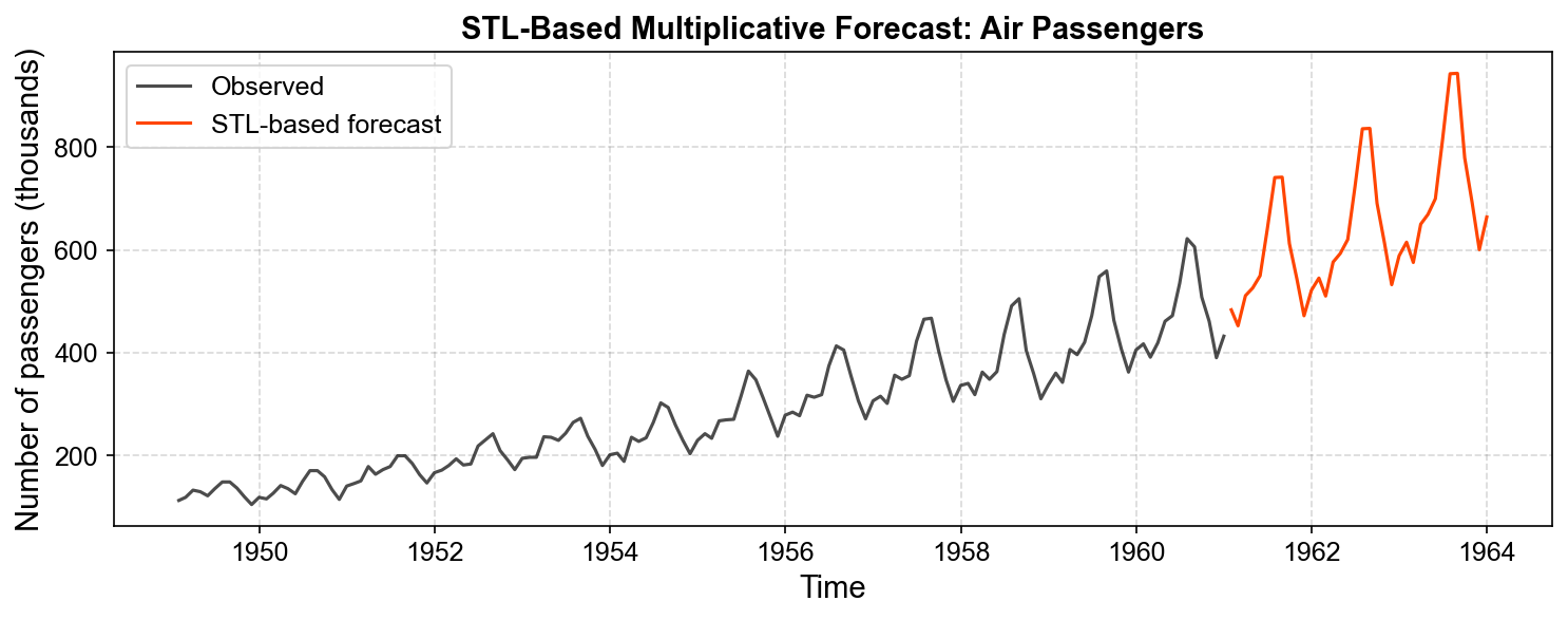
Fig. 3.19 STL-based multiplicative forecasts for the Air Passengers series. The STL decomposition is used to extract a smooth log-trend and stable multiplicative seasonal pattern. A simple linear model extrapolates the log-trend, while the seasonal multipliers are reused in a seasonal-naive fashion. The resulting forecasts preserve proportional seasonal variation around a growing trend, consistent with the multiplicative formulation.#