Remark

Please be aware that these lecture notes are accessible online in an ‘early access’ format. They are actively being developed, and certain sections will be further enriched to provide a comprehensive understanding of the subject matter.

4.1. Time Series Smoothing

4.1.1. Introduction to Smoothing

Time series data often contain substantial noise that obscures underlying trends and cycles, making pattern recognition and forecasting challenging. Smoothing techniques filter out short-term fluctuations to reveal longer-term movements and systematic patterns. Among these methods, the moving average stands as the most widely used approach, offering intuitive interpretation and straightforward implementation [Hyndman and Athanasopoulos, 2018].

When we observe raw time series data—whether stock prices, sensor readings, or sales figures—we typically see a jagged pattern combining several components: a long-term trend showing overall direction, cyclical patterns repeating at regular intervals, and random noise reflecting measurement error and unpredictable influences. Smoothing methods attempt to separate these components, enhancing our ability to identify meaningful signals amid the noise.

Main Concepts of Time Series Smoothing

Trend: The long-term increase or decrease in the data, representing sustained directional movement over an extended period. Trends can be linear (constant rate of change) or nonlinear (accelerating or decelerating growth).

Seasonality: A pattern that repeats at fixed, known intervals—daily cycles in website traffic, weekly patterns in retail sales, or annual fluctuations in energy consumption. Seasonal components reflect calendar effects, weather patterns, or behavioral regularities.

Noise (Residual): The random, unpredictable variation remaining after we account for trend and seasonality. Noise represents genuinely stochastic influences, measurement error, or deterministic factors too complex or irregular to model explicitly.

4.1.2. Simple Moving Average (SMA)

The Simple Moving Average provides the most straightforward smoothing approach: we replace each observation with the average of nearby values within a sliding window. This local averaging attenuates short-term volatility while preserving longer-term patterns, effectively filtering high-frequency noise.

4.1.2.1. Mathematical Formulation

For a time series \(X(t)\) and window size \(k\), we calculate the SMA at time \(t\) as:

(4.1)\[SMA(t) = \dfrac{1}{k} \sum_{i=0}^{k-1} X(t-i)\]

where:

• \(SMA(t)\) denotes the smoothed average value centered at time \(t\).

• \(k\) represents the fixed window size (the count of observations included).

• \(X(t-i)\) is the actual observation from the series at lag \(i\).

• \(t\) indicates the current time step.

This formula averages the current observation with the \(k-1\) most recent previous observations, producing a smoothed value centered at time \(t\).

Window Size Selection

The choice of window size \(k\) represents a fundamental tradeoff between responsiveness and smoothness:

• Smaller \(k\) (e.g., 3-5 periods): The smoothed series responds quickly to recent changes, closely tracking actual data movements. However, significant noise remains, potentially obscuring underlying patterns. We use short windows when recent information matters most—for example, in short-term trading strategies or rapid process control applications.

• Larger \(k\) (e.g., 20-50 periods): The smoothed series exhibits much greater stability, clearly revealing long-term trends. However, it lags substantially behind actual data, responding slowly to genuine changes. We prefer long windows when we want to identify persistent patterns while ignoring short-term volatility—for example, in strategic business planning or long-term trend analysis.

Properties and Behavior

The SMA exhibits several important characteristics:

1. Equal weighting: All observations within the window receive identical weight \(1/k\), regardless of recency. An observation from \(k\) periods ago contributes equally to one from yesterday.

2. Endpoint discontinuities: When we add a new observation to the window while dropping the oldest, the SMA can shift abruptly even when underlying conditions change smoothly.

3. Lag effect: The SMA necessarily trails the actual data, with lag increasing as \(k\) grows. At turning points (peaks or troughs), the SMA continues moving in the previous direction even after the actual series reverses.

4. Trend preservation: While removing noise, SMA preserves linear trends reasonably well, though it dampens the magnitude of changes.

Example 4.1 (Mathematical Calculation (k=3))

We’ll calculate a 3-day Simple Moving Average using NVIDIA (NVDA) stock closing prices to illustrate the mechanics of the sliding window calculation.

Table 4.1 NVIDIA stock prices and 3-day simple moving average calculations for October 27-31, 2025

Date	NVDA Price (\(X(t)\))	3-Day SMA (\(SMA(t)\))	Calculation
2025-10-27 (Day 1)	191.49	N/A	Insufficient data
2025-10-28 (Day 2)	201.03	N/A	Insufficient data
2025-10-29 (Day 3)	207.04	199.85	(191.49 + 201.03 + 207.04)/3
2025-10-30 (Day 4)	202.89	203.65	(201.03 + 207.04 + 202.89)/3
2025-10-31 (Day 5)	202.49	204.14	(207.04 + 202.89 + 202.49)/3

Since \(k=3\), we require three consecutive observations before we can calculate our first SMA value. The calculation proceeds as:

Day 3 (2025-10-29): We now have sufficient data (Days 1-3) to compute our first SMA:

\[\begin{equation*} SMA_{\text{Day 3}} = \dfrac{191.49 + 201.03 + 207.04}{3} = \dfrac{599.56}{3} = 199.85 \end{equation*}\]

Day 4 (2025-10-30): The “moving” aspect emerges here. We shift the window forward: drop Day 1 (191.49), add Day 4 (202.89), and average Days 2-4:

\[\begin{equation*} SMA_{\text{Day 4}} = \dfrac{201.03 + 207.04 + 202.89}{3} = \dfrac{610.96}{3} = 203.65 \end{equation*}\]

Day 5 (2025-10-31): We continue sliding the window: drop Day 2 (201.03), add Day 5 (202.49), and average Days 3-5:

\[\begin{equation*} SMA_{\text{Day 5}} = \dfrac{207.04 + 202.89 + 202.49}{3} = \dfrac{612.42}{3} = 204.14 \end{equation*}\]

Notice how the SMA value changes more gradually than the underlying prices—the averaging process smooths out the day-to-day volatility while capturing the overall movement pattern.

4.1.2.2. Python Example: NVDA Simple Moving Average

We’ll now apply SMAs with two different window sizes to NVIDIA stock data to demonstrate how window selection affects the smoothed series characteristics. A 20-day SMA (approximately one trading month) captures medium-term momentum, while a 50-day SMA (approximately one trading quarter) reveals longer-term trends.

Show code cell source

Hide code cell source

import yfinance as yf

# Fetch data (using the same NVDA example)
df_nvda = yf.download("NVDA", start="2022-11-01", end="2025-11-01", progress=False, auto_adjust=True)

# Calculate SMA (20-day and 50-day)
df_nvda['SMA_20'] = df_nvda['Close'].rolling(window=20).mean()
df_nvda['SMA_50'] = df_nvda['Close'].rolling(window=50).mean()

Loading ITables v2.6.2 from the init_notebook_mode cell... (need help?)

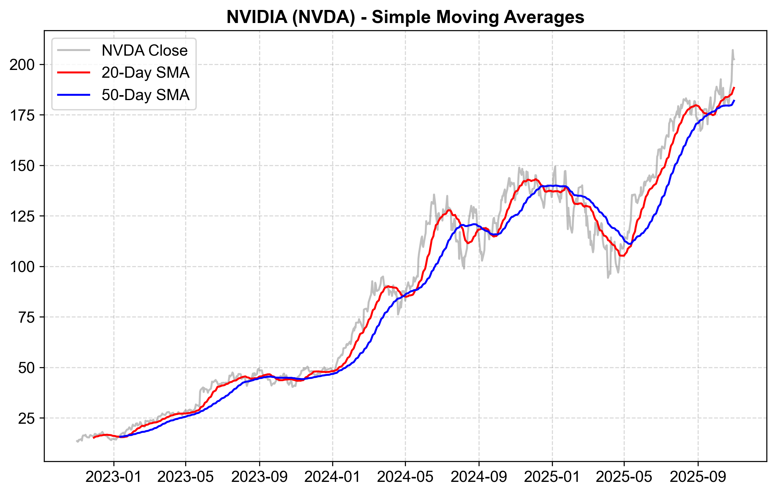
Fig. 4.1 NVIDIA (NVDA) closing prices with 20-day and 50-day simple moving averages from late 2022 through October 2025. The gray line represents actual closing prices, the red line shows the 20-day SMA, and the blue line displays the 50-day SMA.

Fig. 4.1 demonstrates several fundamental behaviors of moving averages applied to NVIDIA stock prices from November 2022 through October 2025. The gray line traces actual daily closing prices, revealing substantial volatility throughout the period. NVIDIA’s dramatic growth during this AI boom period is unmistakable—prices climb from approximately $13 in late 2022 to surpass $200 by late 2025, representing more than a 15-fold increase.

The red 20-day SMA tracks price movements relatively closely while smoothing daily fluctuations. We can observe how it responds to weekly and monthly trends with only modest delay. During the explosive growth phases visible in mid-2023 and throughout 2024, the 20-day average follows prices upward but consistently lags slightly below, confirming sustained upward momentum rather than isolated daily spikes. When prices consolidate—oscillating within a range without clear directional movement (visible in several periods during 2024)—the 20-day SMA settles near the range midpoint, effectively filtering out the noise of daily price reversals while capturing the underlying equilibrium level.

The blue 50-day SMA provides a substantially smoother representation of long-term trend direction, removing nearly all short-term volatility. The overall trajectory becomes unmistakable: from the 2022 lows around $13, through steady acceleration in 2023 (rising from roughly $40 to $90), explosive expansion throughout 2024 (climbing from $90 to peaks near $140, then consolidating), and a final surge to the $180-190 range by late 2025. This long-term average clarifies the sustained multi-year uptrend despite numerous intermediate corrections.

However, the 50-day SMA’s extreme smoothness comes at the cost of substantial lag. We can observe several instances where prices peak and begin reversing—most notably the corrections in late 2024 around August-September where prices dropped from approximately $140 to below $100—yet the 50-day SMA continues rising for several weeks afterward, only reversing direction well after the actual trend shift occurred. This lag illustrates a critical limitation: by the time the 50-day average signals a trend change, much of the move has already transpired.

Moving Average Interactions

Fig. 4.1 reveals several periods where the two moving averages converge or cross, which technical analysts interpret as significant signals. In early 2023, we can observe the 20-day SMA crossing above the 50-day SMA as both accelerate upward together—a “golden cross” pattern suggesting strengthening momentum. The gap between the two averages expands during strong trends (2023 mid-year, early 2024, late 2025), indicating not just rising prices but accelerating momentum. Conversely, when the averages converge (visible in the 2024 mid-year consolidation around $120-140), it suggests indecision or trend exhaustion.

The relationship between actual prices and the moving averages also provides context. When prices extend far above both averages—as in the surges past $130 in mid-2024 and above $200 in late 2025—the market is “overextended” relative to recent norms, potentially suggesting either exceptionally strong momentum or increased vulnerability to pullbacks. When prices fall back toward the moving averages, these levels often act as support where buying interest emerges, visible in several bounces throughout the period.

Practical Insights

For NVIDIA specifically, the moving averages confirm what the raw price data suggests: this has been an extraordinarily strong, sustained uptrend with only brief, shallow corrections. The 20-day SMA spent most of the three-year period rising steadily with few significant reversals, while the 50-day SMA exhibited an almost uninterrupted ascent from $20 to $185. Such persistent trends are unusual—most stocks experience more frequent mean reversion—highlighting NVIDIA’s exceptional fundamental momentum during the AI investment boom.

The chart also illustrates why moving averages work better for some data than others. NVIDIA’s strong trending behavior makes moving averages useful trend-following tools—staying above the 50-day SMA would have kept investors positioned through most of the spectacular gains. However, for more cyclical or mean-reverting stocks, moving averages generate more whipsaw signals as prices repeatedly cross above and below the averages without establishing clear trends.

4.1.3. Weighted Moving Average (WMA)

The Weighted Moving Average (WMA) addresses a fundamental limitation of the Simple Moving Average by recognizing that not all observations within a time window carry equal informational value. Recent observations typically provide more relevant information about current conditions than older data points. The WMA assigns linearly decreasing weights within a fixed window, giving greater importance to recent data while maintaining the conceptual simplicity of a defined lookback period.

The WMA occupies middle ground between the SMA (which treats all window observations equally) and the Exponential Moving Average (which applies exponentially decreasing weights across infinite history). This intermediate position offers advantages in specific applications where we want enhanced responsiveness without committing to EMA’s infinite memory structure.

Conceptual Framework: We assign weights that decrease in arithmetic progression, with the most recent observation receiving the highest weight. For a 3-day window, we might use weights of 3, 2, and 1 for days \(t\), \(t-1\), and \(t-2\) respectively. This weighting scheme ensures that today’s price influences the average three times more strongly than the price from two days ago—a reasonable approximation of how information relevance decays with time.

Use Cases: The WMA proves most valuable when we need greater responsiveness than the SMA provides but want precise control over the lookback period without the complexity of EMA’s infinite memory. Applications include medium-term trend following, technical analysis where specific window lengths have conventional significance (e.g., 20-day trading month), and situations where we want complete data obsolescence after \(N\) periods rather than EMA’s gradual decay.

Comparison: WMA vs. EMA

• Memory and Computational Structure:

  • WMA: Maintains finite memory with linear weighting. The oldest data point drops completely from the calculation after \(N\) periods, creating a sharp cutoff. We must store and process the full window of past values for each calculation, making it computationally similar to SMA but with the added complexity of weight multiplication.

  • EMA: Theoretically maintains infinite memory with exponential decay. However, it’s computationally efficient because we only need the previous EMA value and the current observation—no historical data storage required. The recursive formulation \(EMA_t = \alpha \cdot X_t + (1-\alpha) \cdot EMA_{t-1}\) makes real-time calculation trivial.

• Responsiveness Characteristics:

  • WMA: Provides intermediate responsiveness between SMA and EMA. The linear weighting scheme creates moderate sensitivity to recent price changes. When prices shift suddenly, the WMA adjusts faster than SMA because recent observations dominate, but slower than EMA because older observations still contribute with diminishing but substantial weights.

  • EMA: Exhibits the highest responsiveness to recent changes due to exponential decay, making it preferred for short-term trading strategies where rapid adaptation to new information matters most. However, this responsiveness comes at the cost of never fully forgetting old data—even ancient observations contribute microscopically to current EMA values.

Practical Tradeoffs: For longer window lengths (e.g., 20-50 periods), the practical difference between WMA and SMA often proves minimal because the enhanced weighting of recent observations in WMA gets averaged out over the longer period. The WMA shines most clearly with shorter windows (3-10 periods) where the linear weighting creates meaningful differentiation from equal weighting.

4.1.3.1. Mathematical Formulation

For a window of size \(N\), we assign weights \(w_t, w_{t-1}, \ldots, w_{t-N+1}\) to the data points in the window. The most common form is the Linear Weighted Moving Average, where the weight for the current observation is \(N\), the previous observation is \(N-1\), continuing down to 1 for the oldest observation in the window.

For a time series \(X(t)\):

(4.2)\[\begin{equation} WMA_t = \dfrac{\sum_{i=0}^{N-1} (N-i) \times X(t-i)}{\sum_{i=0}^{N-1} (N-i)} \end{equation}\]

We can simplify the denominator using the triangular number formula \(\sum_{i=1}^{N} i = \dfrac{N(N+1)}{2}\):

(4.3)\[\begin{equation} WMA_t = \dfrac{N \cdot X(t) + (N-1) \cdot X(t-1) + \cdots + 1 \cdot X(t-N+1)}{\dfrac{N(N+1)}{2}} \end{equation}\]

Where:

• \(X(t)\) represents the current price or value

• \(N\) is both the window size and the weight assigned to the most recent observation

• \(\dfrac{N(N+1)}{2}\) is the sum of weights (the \(N\)th triangular number)

Example 4.2 (Mathematical Calculation: 3-Day WMA)

We’ll calculate the 3-Day WMA for NVDA data at Day 5 to demonstrate how linear weighting affects the result compared to equal weighting (SMA).

Weight Assignment:

For a 3-day window (\(N=3\)):

• Current Day (\(t\)): Weight = 3

• Previous Day (\(t-1\)): Weight = 2

• Day before (\(t-2\)): Weight = 1

• Total Sum of Weights: \(3+2+1 = 6\) (or equivalently, \(\dfrac{3(3+1)}{2} = 6\))

Data and Weighted Values:

Table 4.2 Weight assignments and weighted price calculations for 3-day WMA computation on NVDA stock

Date	Weight (\(w\))	NVDA Price (\(X_t\))	\(w \times X_t\)
Day 3	1	207.04	207.04
Day 4	2	202.89	405.78
Day 5	3	202.49	607.47

Calculation:

\[\begin{equation*} WMA_{\text{Day 5}} = \dfrac{(3 \times 202.49) + (2 \times 202.89) + (1 \times 207.04)}{3+2+1} \end{equation*}\]

\[\begin{equation*} WMA_{\text{Day 5}} = \dfrac{607.47 + 405.78 + 207.04}{6} = \dfrac{1220.29}{6} = \mathbf{203.38} \end{equation*}\]

Comparison for Day 5:

• SMA (Equal Weight): 204.14 (highest value—the older Day 3 price of 207.04 pulls the average upward)

• WMA (Linear Weight): 203.38 (intermediate value—recent prices receive more influence)

• Actual Day 5 Price: 202.49 (current observation)

The WMA’s value of 203.38 lies between the SMA and the current price because it weights the recent prices (202.49 and 202.89) more heavily than the older price (207.04). This demonstrates how linear weighting provides faster adaptation to recent price movements compared to equal weighting, though the difference appears modest for such a short window.

If we examine the contribution breakdown:

• Day 5 (202.49) contributes 607.47/1220.29 ≈ 49.8% of the weighted total

• Day 4 (202.89) contributes 405.78/1220.29 ≈ 33.2%

• Day 3 (207.04) contributes 207.04/1220.29 ≈ 17.0%

Under equal weighting (SMA), each day would contribute exactly 33.3%. The WMA’s structure gives nearly half the total weight to just the most recent observation.

4.1.3.2. Python Example: NVIDIA WMA Analysis

Pandas does not provide a built-in .wma() method like it does for exponential weighting (.ewm()), but we can construct the WMA using .rolling().apply() with a custom function.

Show code cell source

Hide code cell source

import numpy as np

# Define a function to calculate WMA for a given window
def linear_wma(window):
    weights = np.arange(1, len(window) + 1)
    return np.dot(window, weights) / weights.sum()

import yfinance as yf

# Fetch data (using the same NVDA example)
df_nvda = yf.download("NVDA", start="2022-11-01", end="2025-11-01", progress=False, auto_adjust=True)

# Calculate SMA (20-day)
df_nvda['SMA_20'] = df_nvda['Close'].rolling(window=20).mean()

# Calculate Weighted Moving Average (WMA)
# We use a rolling window of 20, applying our custom WMA function
df_nvda['WMA_20'] = df_nvda['Close'].rolling(window=20).apply(linear_wma)

Loading ITables v2.6.2 from the init_notebook_mode cell... (need help?)

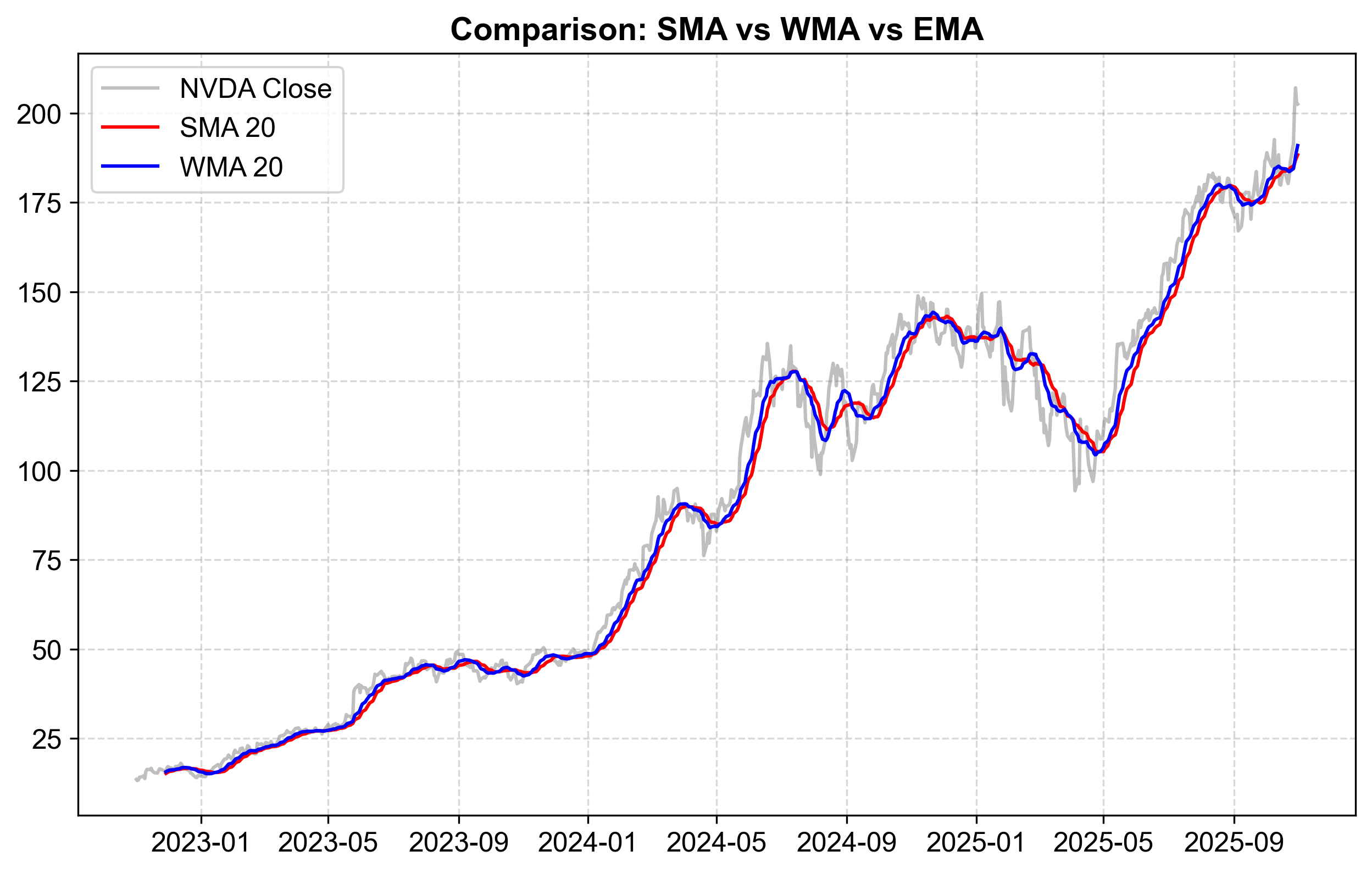
Fig. 4.2 NVIDIA stock price comparison with 20-day SMA (red) and WMA (blue) from late 2022 through October 2025. The gray line represents daily closing prices, revealing the extreme volatility characteristic of the AI boom period.

Fig. 4.2 reveals a surprising finding: despite the theoretical advantages of linear weighting, the 20-day WMA (blue) and 20-day SMA (red) track almost identically throughout the entire three-year period. The two lines appear virtually superimposed, making them difficult to distinguish visually. This near-perfect overlap demonstrates an important practical reality about moving averages: for moderate-to-long window lengths (20 periods or more), the choice between equal and linear weighting often makes negligible difference in practice.

The minimal differentiation between SMA and WMA at a 20-day window occurs because:

1. Averaging effect: With 20 observations, even though the WMA weights the most recent day at 20× the oldest day, this differential gets averaged across a large number of intermediate observations with intermediate weights. The cumulative effect smooths out much of the intended responsiveness advantage.

2. Strong trend dominance: NVIDIA’s price trajectory during this period exhibits sustained, powerful trends rather than frequent reversals. In strongly trending markets, both SMA and WMA lag behind prices in similar ways because the fundamental issue—backward-looking averaging—affects both methods equally.

3. High volatility: Daily price swings in NVIDIA stock are substantial (visible in the gray line’s jagged appearance). This high-frequency volatility affects both averages similarly, as both methods average over the same 20-day period regardless of weighting scheme.

We would observe more meaningful separation between SMA and WMA under conditions such as:

• Shorter windows (5-10 days): The weight differential becomes more pronounced, making WMA noticeably more responsive

• Trend reversals: When prices peak and reverse direction, WMA should theoretically detect the shift faster

• Lower volatility: When daily fluctuations are smaller relative to trend changes, the weighting scheme’s influence becomes more visible

Both moving averages exhibit substantial lag behind actual prices during the sustained uptrend visible from early 2023 through mid-2024. When prices climb from approximately \(40 to \)140, both the SMA and WMA consistently trail below, typically lagging by $5-15. This lag is characteristic of all backward-looking moving averages in trending markets—they necessarily average past prices, which in an uptrend are lower than current prices.

During consolidation periods—most notably in the $120-140 range throughout mid-2024—both moving averages converge closer to actual prices and become more useful as support/resistance indicators. When prices lack a clear directional trend, the averaging process provides valuable information about the range midpoint rather than merely lagging behind a moving target.

Practical Implications

For practitioners considering whether to implement WMA over SMA:

• Computational cost: WMA requires storing the full 20-day window plus applying custom weighting logic, while SMA uses simpler arithmetic. For real-time systems processing thousands of securities, this overhead matters.

• Interpretability: SMA’s equal weighting makes it easier to explain and interpret. When we say “20-day average,” stakeholders understand we’re averaging 20 days equally. WMA’s linear weighting requires additional explanation about why recent days matter more.

• Practical benefit: This chart suggests that for 20-day windows, the added complexity of WMA provides minimal practical advantage over SMA. The theoretical responsiveness benefit fails to materialize in meaningful ways for this application.

When WMA Adds Value

Based on this analysis, we should consider WMA most seriously when:

• Using shorter windows (3-10 periods) where weight differentials create visible differences

• Analyzing mean-reverting rather than trending data where rapid reversal detection matters

• Working with lower-frequency data (weekly, monthly) where individual observations carry more distinct information

• Building trading systems where even small edges compound over many trades

For the common application of 20-50 day moving averages in financial markets, the SMA’s simplicity and computational efficiency make it the pragmatic choice unless specific backtesting demonstrates that WMA’s marginal responsiveness advantage translates to measurably improved performance.

4.1.4. Exponential Moving Average (EMA)

While the Simple Moving Average assigns equal weight to all observations within its window, the Exponential Moving Average (EMA) applies a weighting scheme that decreases exponentially for older data points. This approach places progressively greater significance on recent observations, making the EMA substantially more responsive to new information—a characteristic particularly valued by traders seeking to identify trend reversals and momentum shifts early.

The exponential weighting structure represents a fundamental departure from fixed-window methods. Rather than maintaining a sharp cutoff where observations suddenly drop from the calculation (as in SMA and WMA), the EMA theoretically incorporates all historical data with weights that decay exponentially. In practice, very old observations contribute negligibly, but mathematically every past value influences the current EMA to some degree.

Comparison: SMA vs. EMA

• SMA Characteristics:

  • Responds slowly to price changes due to equal weighting of all window observations

  • Provides greater smoothing, filtering out more noise

  • Better suited for identifying established long-term trends and support/resistance levels

  • Less prone to false signals during consolidation, but slower to confirm genuine trend changes

• EMA Characteristics:

  • Reacts faster to price changes due to exponential weighting favoring recent observations

  • Maintains less smoothing, preserving more responsiveness to current conditions

  • Better suited for short-term trend identification and momentum trading

  • More likely to generate false signals during choppy, range-bound markets but catches trend reversals earlier

The choice between SMA and EMA depends on our trading or analysis timeframe and tolerance for false signals versus lag in trend detection.

4.1.4.1. Single Exponential Smoothing (Standard EMA)

The standard EMA represents the foundational form used extensively in technical analysis and time series forecasting. It assumes the data fluctuate around a moving level without consistent trend or seasonality—appropriate for many financial markets where short-term movements lack clear directional bias.

We calculate each new smoothed value as a weighted average of the current observation and the previous smoothed value. The smoothing parameter \(\alpha\) determines the balance between responsiveness and stability:

• High \(\alpha\) (close to 1): The system reacts quickly to recent changes, giving heavy weight to the current observation. This creates minimal smoothing and maximum responsiveness—suitable for very short-term analysis but vulnerable to noise.

• Low \(\alpha\) (close to 0): The system retains substantial “memory” of past values, changing slowly. This creates heavy smoothing that filters noise effectively but lags significantly behind genuine changes.

Mathematical Formulation:

For a time series \(X(t)\) and smoothing parameter \(\alpha\) where \(0 \leq \alpha \leq 1\) [Brown, 2004, Hyndman and Athanasopoulos, 2018]:

(4.4)\[\begin{equation} S(t) = \alpha X(t) + (1 - \alpha) S(t-1) \end{equation}\]

where,

• \(S(t)\): The new smoothed level (EMA) at time \(t\)

• \(\alpha X(t)\): The correction term pulling the average toward the current actual value

• \((1 - \alpha) S(t-1)\): The memory term preserving a portion of the previous average

This recursive formulation reveals the EMA’s computational elegance: we need only the previous EMA and the current observation, not the entire historical dataset.

The Smoothing Factor (\(\alpha\))

For equivalence with an \(N\)-day moving average, we commonly approximate the smoothing factor as:

(4.5)\[\alpha = \dfrac{2}{N + 1}\]

This formula ensures that the EMA’s effective lookback roughly corresponds to an \(N\)-day window, though the exponential weighting creates different behavior than true \(N\)-day equal weighting.

Example 4.3 (Mathematical Calculation: 3-Day EMA)

We’ll demonstrate how the EMA responds more quickly than the SMA using the same NVDA data with a 3-day window.

Smoothing Factor: For a 3-day EMA: \(\alpha = \dfrac{2}{3+1} = 0.5\)

Table 4.3 NVIDIA stock prices and 3-Day EMA calculations for October 27-31, 2025

Date	NVDA Price (\(X_t\))	3-Day SMA
Day 1	191.49	-
Day 2	201.03	-
Day 3	207.04	199.85
Day 4	202.89	203.65
Day 5	202.49	204.14

Step 1: Initialization (Day 3)

We cannot calculate an EMA without a previous EMA value \(S(t-1)\). For the initial point, we seed the EMA with the first available SMA:

\[\begin{equation*} EMA_{\text{Day 3}} = SMA_{\text{Day 3}} = 199.85 \end{equation*}\]

Step 2: Calculate Day 4 EMA

Applying the formula \(S(t) = \alpha X(t) + (1-\alpha) S(t-1)\):

\[\begin{equation*} EMA_{\text{Day 4}} = (0.5 \times 202.89) + (0.5 \times 199.85) \end{equation*}\]

\[\begin{equation*} EMA_{\text{Day 4}} = 101.445 + 99.925 = \mathbf{201.37} \end{equation*}\]

Step 3: Calculate Day 5 EMA

\[\begin{equation*} EMA_{\text{Day 5}} = (0.5 \times 202.49) + (0.5 \times 201.37) \end{equation*}\]

\[\begin{equation*} EMA_{\text{Day 5}} = 101.245 + 100.685 = \mathbf{201.93} \end{equation*}\]

Comparative Analysis:

Method	Day 5 Value	Distance from Actual (202.49)
Actual Price	202.49	0.00
EMA	201.93	0.56
WMA	203.38	0.89
SMA	204.14	1.65

The EMA tracks closest to the actual Day 5 price, demonstrating its superior responsiveness. The SMA overshoots significantly because it remains “anchored” to the higher prices from Days 3-4, giving them equal weight to the recent decline. The EMA, by contrast, weights Day 5 (202.49) and Day 4 (202.89) most heavily, allowing it to adapt faster to the downward movement.

Exponential Weight Structure:

With \(\alpha = 0.5\), the effective weights in the Day 5 EMA are:

• Day 5: 50% (direct contribution via \(\alpha\))

• Day 4: 25% (contributes 50% of Day 4’s 50% influence on Day 4 EMA)

• Day 3: 12.5% (exponentially decaying)

• Days 1-2: 12.5% combined (residual from initialization)

This exponential decay ensures recent observations dominate while older values fade rapidly—the core advantage over equal weighting.

4.1.4.2. Python Example: NVIDIA EMA Analysis

Show code cell source

Hide code cell source

import yfinance as yf
import pandas as pd
import matplotlib.pyplot as plt

# 1. Fetch Data
# We download NVDA data. auto_adjust=True ensures we use data adjusted for splits/dividends.
df = yf.download("NVDA", start="2022-11-01", end="2025-11-01", progress=False, auto_adjust=True)

# 2. Calculate Simple Moving Averages (SMA)
# Using .rolling() which gives equal weight to all items in the window
df['SMA_20'] = df['Close'].rolling(window=20).mean()
df['SMA_50'] = df['Close'].rolling(window=50).mean()

# 3. Calculate Exponential Moving Averages (EMA)
# Using .ewm() (Exponential Weighted Functions)
# span=20 calculates alpha automatically as 2/(20+1)
# adjust=False calculates the EMA recursively (standard trading method)
df['EMA_20'] = df['Close'].ewm(span=20, adjust=False).mean()
df['EMA_50'] = df['Close'].ewm(span=50, adjust=False).mean()

Loading ITables v2.6.2 from the init_notebook_mode cell... (need help?)

Fig. 4.3 NVIDIA stock comparison of 20-day SMA (red dashed line) versus 20-day EMA (green solid line) from late 2022 through October 2025. The gray line represents daily closing prices, revealing extreme volatility throughout the AI boom period.

The figure demonstrates the behavioral differences between SMA and EMA applied to NVIDIA’s dramatic three-year price journey. The most striking observation: despite theoretical differences in weighting schemes, the 20-day SMA (red dashed) and 20-day EMA (green solid) track remarkably closely throughout most of the period, often appearing nearly superimposed.

Early Period Similarity (Late 2022 - Mid 2023): From the chart’s beginning through mid-2023, as prices climb from approximately $13 to $45, both moving averages follow nearly identical paths. The exponential weighting advantage of the EMA produces minimal visible differentiation from the SMA’s equal weighting at this timescale. Both averages lag similarly behind the rising prices, trailing by roughly $2-5 during steady uptrends.

Responsiveness During Acceleration (Mid 2023 - Early 2024): As NVIDIA enters explosive growth from $45 to $90 and then to $125, we begin observing subtle but meaningful differences. The EMA (green) occasionally sits slightly higher than the SMA (red) during strong uptrends. This makes intuitive sense—the EMA weights recent high prices more heavily, pulling it upward faster than the SMA which must “drag along” older lower prices with equal weight. However, the magnitude remains modest, typically $1-3 of separation—meaningful for trading but not dramatically different from a visual perspective.

Divergence During Volatility (2024 Consolidation): The most pronounced EMA-SMA separation occurs during the volatile consolidation period in mid-to-late 2024, when prices oscillate between $110 and $145. During sharp reversals—particularly the correction from $140 to $100 visible around August-September 2024—the EMA responds slightly faster to the downturn. We can observe the green EMA line beginning to curve downward marginally ahead of the red SMA line, confirming the EMA’s theoretical advantage in detecting trend changes earlier.

Following this correction, as prices recover from $100 back toward $130 in late 2024, the EMA again leads slightly on the upside, reaching recovery levels a few days before the SMA. This pattern—EMA leading at turning points—represents its core value proposition for trend-following strategies.

Final Surge (Late 2025): In the chart’s final months, as NVIDIA surges from $140 to above $185, both averages again converge closely. The powerful, sustained uptrend creates conditions where both methods produce similar results—when directional movement dominates over noise, the choice of weighting scheme matters less.

Quantitative Assessment

Throughout the three-year period, the typical EMA-SMA separation ranges from $0 to $4, with occasional spikes to $5-6 during extreme volatility. Given NVIDIA’s price scale ($15-$200), this represents roughly 0-2% difference—significant for active traders managing risk tightly, but modest in the context of the stock’s 1,300% gain over the period.

Practical Implications

The near-overlap of 20-day SMA and EMA suggests several practical insights:

1. Window length matters more than weighting: For 20-day windows, both methods smooth similarly. The distinction becomes more pronounced with shorter windows (5-10 days) where EMA’s responsiveness advantage amplifies.

2. Trend dominance: In strongly trending markets like NVIDIA’s 2023-2025 run, both methods lag persistently behind prices. The fundamental issue—backward-looking averaging—affects both equally. Neither can “predict” continuation; both merely confirm established trends.

3. Computational considerations: EMA’s recursive calculation (\(S_t = \alpha X_t + (1-\alpha)S_{t-1}\)) requires minimal memory and computation compared to SMA’s need to store and average 20 values. For systems monitoring thousands of securities in real-time, this efficiency advantage matters despite producing similar visual results.

4. Trading signal generation: Technical traders often use moving average crossovers (when fast MA crosses slow MA) as trade signals. The chart suggests that using 20-day EMA versus 20-day SMA would generate nearly identical signals—the crossovers with a 50-day average would occur within days of each other.

When EMA Advantages Materialize

Based on this analysis, we should expect more substantial EMA benefits when:

• Using shorter windows (5-12 days) where weight differences amplify

• Trading mean-reverting rather than trending securities where rapid reversals occur frequently

• Operating in choppy, range-bound markets where early reversal detection provides edge

• Requiring real-time computational efficiency for large-scale monitoring systems

For the common application of 20-50 day moving averages in equity analysis, the choice between SMA and EMA often comes down to personal preference and existing infrastructure rather than dramatically different analytical outcomes.