Remark
Please be aware that these lecture notes are accessible online in an ‘early access’ format. They are actively being developed, and certain sections will be further enriched to provide a comprehensive understanding of the subject matter.
1.5. What Are ACF and PACF?#
The Autocorrelation Function (ACF) and Partial Autocorrelation Function (PACF) are fundamental diagnostic tools for understanding the internal structure of time series data. They allow us to visualize how observations in a time series correlate with their own past values, answering the central question: How does the past relate to the present?
Both plots display correlation coefficients ranging from −1 to +1 on the vertical axis and time lags on the horizontal axis. The key distinction between them lies in the type of correlation being measured. ACF measures total correlation (including indirect effects), while PACF isolates only the direct relationship between observations after accounting for intermediate values.
1.5.1. The ACF Plot: Understanding Overall Dependence#
The Autocorrelation Function (ACF) measures the linear correlation between a time series and lagged versions of itself. At lag \(k\), the ACF compares the current observation \(Y_t\) with the observation from \(k\) periods ago, \(Y_{t-k}\). Mathematically, this is expressed as [Chiang et al., 2024, Statsmodels Developers, 2023]:
When you look at an ACF plot, the horizontal axis represents different lags (time distances), and each vertical bar represents the strength of correlation at that lag. The bar height tells you the correlation coefficient: values near +1 indicate strong positive correlation, values near −1 indicate strong negative correlation, and values near 0 indicate weak or no relationship. The lag 0 always equals 1.0 (a variable perfectly correlates with itself), though this is typically not shown on the plot.
The shaded blue region in the middle represents the confidence bands, typically set at ±2 standard errors, which corresponds to a 95% confidence level. Bars that fall entirely within this band are considered statistically insignificant—they could easily arise from random chance. Bars that cross beyond the band indicate correlations that are unlikely to be due to randomness alone and therefore represent meaningful relationships in your data.
1.5.1.1. What Different ACF Patterns Tell You#
When you examine an ACF plot, several visual patterns reveal important characteristics of your time series. A series might show rapid decay, where bars quickly shrink in height and fall within the confidence bands after just a few lags. This suggests the series has weak dependence on its distant past—knowing what happened 10 or 20 periods ago doesn’t help much in predicting the current value. Conversely, a series might exhibit slow decay, where bars remain large and significant even at large lags, indicating that the series has long-term memory. In such cases, observations far in the past continue to influence current values.
Another important pattern is cyclical or seasonal behavior, where you observe repeating spikes at regular intervals. For example, with monthly data, strong positive spikes might appear at lags 12, 24, and 36, indicating that each month tends to resemble the same month from previous years. This is the hallmark of seasonal data. Finally, if the ACF bars oscillate between positive and negative values, alternating above and below zero, this often suggests the series exhibits mean-reversion, where values tend to bounce back toward a long-term average rather than drift persistently in one direction.
1.5.1.2. Example: Monthly Temperature Data with Strong Seasonality#
To make these concepts concrete, consider a real-world example: monthly average temperature data from Columbia, Missouri. The data spans from 2020 to 2024, sourced from https://open-meteo.com/, with daily temperatures aggregated to monthly means measured in degrees Celsius. This dataset is particularly useful for learning because temperature naturally exhibits strong seasonality—warm summers and cold winters repeat predictably each year.
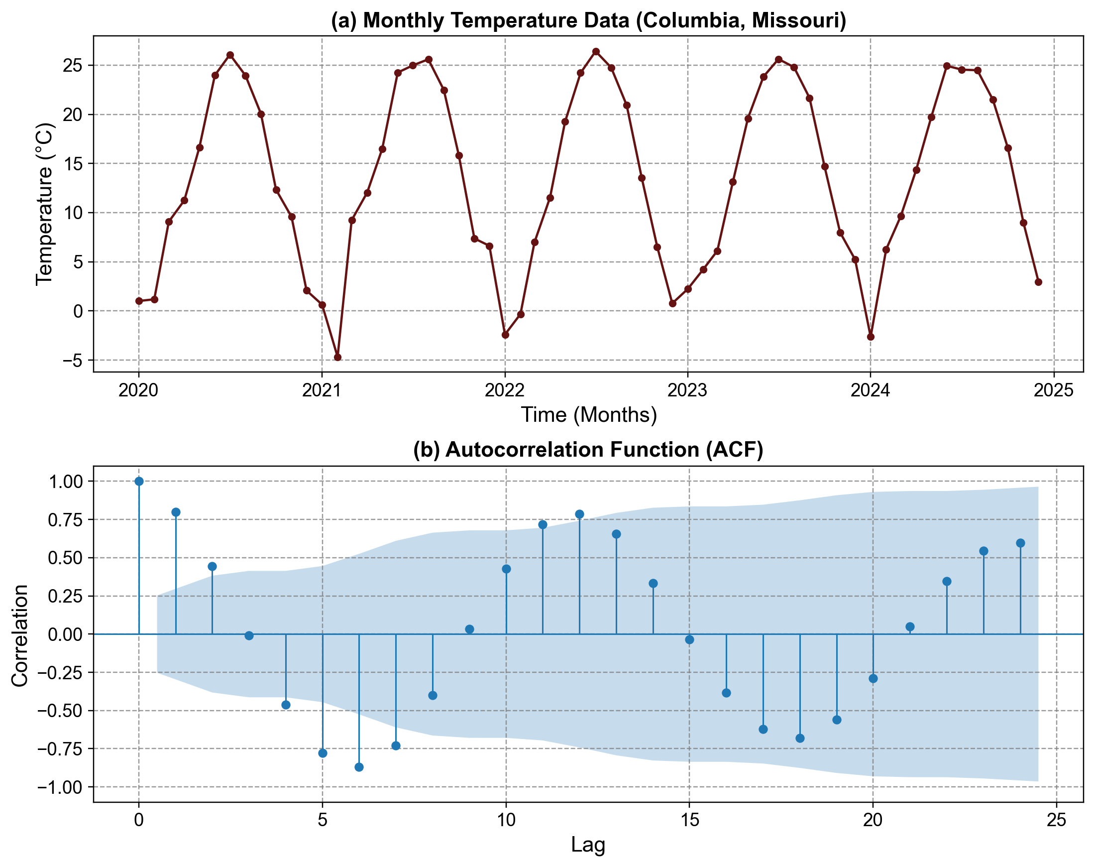
Fig. 1.9 Monthly Temperature Time Series and ACF: (a) Monthly Temperature Data showing clear annual seasonality, (b) Autocorrelation Function revealing strong seasonal patterns#
When we examine the ACF plot for this temperature series, we immediately notice something striking: instead of bars decaying smoothly toward zero, they follow a wavering, sinusoidal pattern. This wavelike behavior is the telltale signature of seasonal data.
Looking more closely at the structure, the tallest positive bars appear at lags 12 and 24. This makes intuitive sense: lag 12 represents “one year ago,” and indeed, January’s temperature is very similar to January from the previous year, with a correlation of approximately 0.80. The temperature in July is similarly correlated with July from the year before. This 12-month periodicity repeats at lag 24 as well, confirming the pattern holds across multiple years.
But there is more happening in the plot. Between these positive peaks, we see significant negative dips, most notably at lag 6. A negative correlation at lag 6 reveals seasonal opposition: summer months are warm while winter months are cold. If we compare June’s temperature (around 24°C, peak summer) with December’s temperature (around 2°C, peak winter), they are strongly negatively correlated (roughly -0.75). This opposite relationship emerges because they represent opposite seasons, six months apart.
The critical observation here is that this ACF does not decay to zero quickly. Even at lag 20, the correlations remain substantial and structured. This persistent pattern indicates that the temperature series is non-stationary—it doesn’t settle into random noise around a constant mean. Instead, it exhibits strong, repeating structure. From a modeling perspective, this tells us that a simple model that ignores seasonality will perform poorly. The model must account for the predictable annual cycle.
Note
We will cover stationary and non-stationary time series in the next chapters.
1.5.2. The PACF Plot: Isolating Direct Relationships#
The Partial Autocorrelation Function (PACF) measures a different type of correlation. It captures the correlation between \(Y_t\) and \(Y_{t-k}\) after removing the effects of all intermediate lags (\(Y_{t-1}, Y_{t-2}, \ldots, Y_{t-k+1}\)) [Chiang et al., 2024, Statsmodels Developers, 2023]. Think of it as a more refined question: Does knowing \(Y_{t-k}\) help me predict \(Y_t\), given that I already know all the values in between?
To illustrate this distinction, imagine you want to predict tomorrow’s temperature (a simple AR example: \(Y_t = Y_{t-1} + \text{noise}\), where today’s temperature is roughly yesterday’s plus some random variation). The ACF would show high correlation at lag 1 (today correlates with yesterday) and still show moderate correlation at lag 2 (because yesterday correlated with the day before), lag 3, and beyond. The correlation decays gradually. However, the PACF would show a large spike at lag 1 but near-zero values at lags 2 and beyond. Why? Because once you know yesterday’s value, knowing the day before adds no new information—the day before’s influence is already captured in yesterday’s value.
The PACF plot has the same visual format as the ACF: bars represent lags, the shaded region is the confidence band, and bars crossing outside the band indicate statistically significant relationships. However, the interpretation is more specific. A sharp cutoff in PACF—where you see a few tall bars followed by silence (all bars within the band)—indicates that the system has short memory. Only the most recent few lags matter directly. In contrast, a gradual decay in PACF is less common and usually indicates a more complex underlying structure.
1.5.2.1. Example: Synthetic Daily Stock Returns#
To understand PACF in a different context, consider synthetic daily stock returns generated from a random normal distribution with mean 0 and 2% standard deviation. This data simulates an efficient financial market where past returns do not predictably influence future returns. Unlike temperature, stock returns show no seasonal pattern.
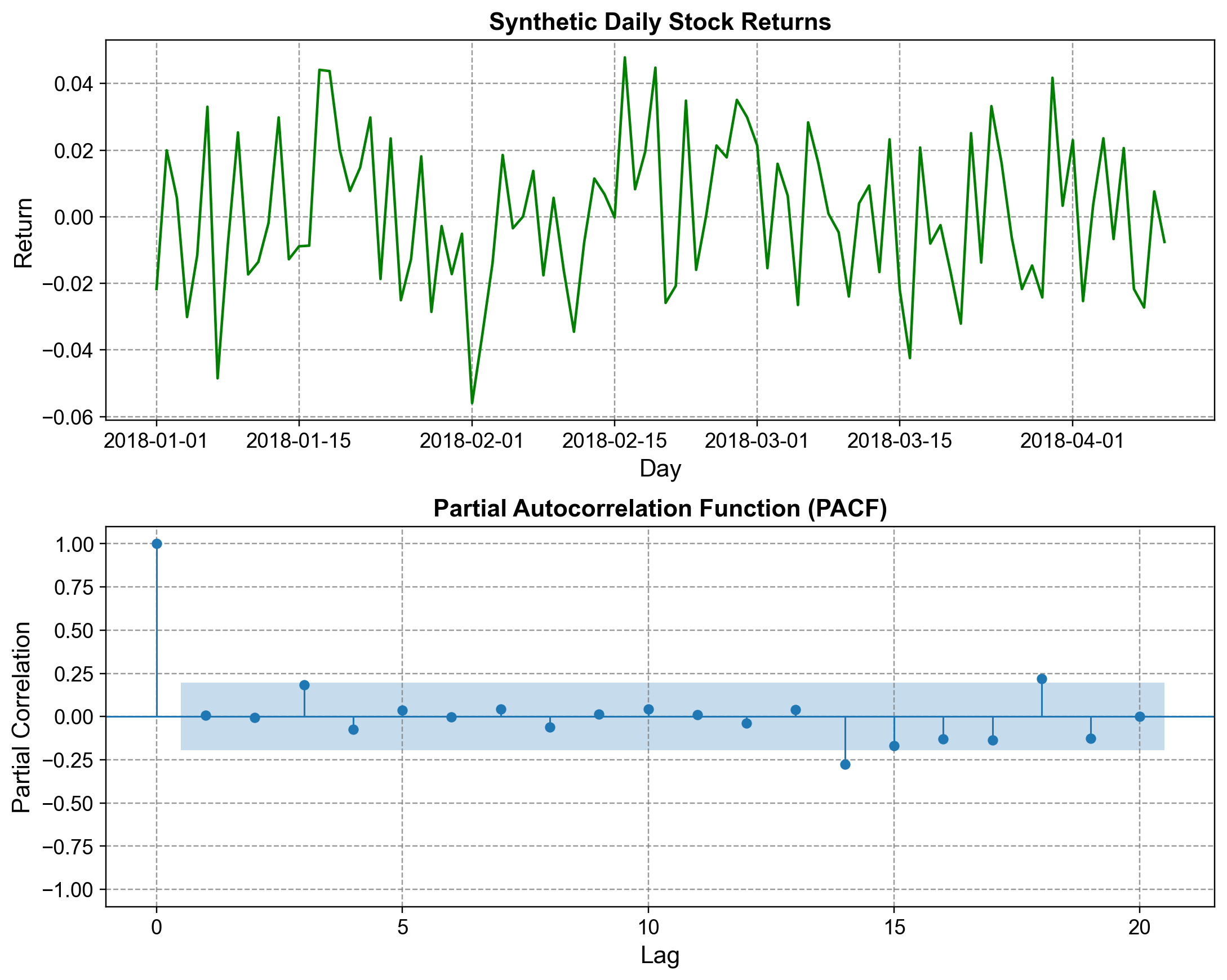
Fig. 1.10 Daily Stock Returns Time Series and PACF: (a) Synthetic daily stock returns showing no systematic patterns, (b) Partial Autocorrelation Function revealing absence of predictive structure#
When we compute the PACF for this returns series, examining lags up to 20 (representing about four weeks of trading days), we observe a strikingly different pattern from the temperature ACF. Almost all the bars fall cleanly within the confidence bands. Lag 0 is not shown, but conceptually it is 1.0. At lag 1, the bar sits just barely above zero but remains comfortably inside the confidence band, indicating no statistically significant partial autocorrelation. The same is true for lags 2 through 20. A few scattered bars occasionally touch or slightly cross the band boundary (perhaps around lag 3 or lag 8), but these are best interpreted as random fluctuations rather than systematic patterns.
What is conspicuously absent here is a sharp cutoff—that is, a prominent spike followed by silence. If this were a truly autoregressive process (say, AR(1)), we would expect a large spike at lag 1 and then zeros everywhere else. Instead, we see no such structure. The PACF reveals that yesterday’s return provides almost no unique predictive information about today’s return. Even if there were a tiny correlation, it is far below the threshold of statistical significance. This pattern is characteristic of white noise or near-random-walk behavior, which aligns with the efficient market hypothesis: prices adjust so quickly to information that past returns cannot be reliably used to forecast future returns.
The absence of PACF structure has important practical implications. It suggests that any autoregressive model fitted to this data would be spurious. The best model is simply a constant (the mean return) plus random noise. Attempting to trade based on perceived momentum or reversal patterns detected in such a series would likely fail once you account for transaction costs and the true randomness of the process.
1.5.3. Comparing ACF and PACF#
Now that we have examined both functions, it is helpful to step back and compare them systematically. The ACF measures total correlation, which includes both direct effects and indirect effects that ripple through intermediate lags. It answers the question “Is this lag correlated with the present?” without worrying about how or why. The PACF measures direct correlation, filtering out the contributions of intermediate lags. It answers the more specific question “Does this lag provide additional predictive information beyond what we already know from closer lags?”
For detecting seasonality and trends, the ACF is your primary tool. Seasonal patterns show up as repeating spikes at fixed intervals (every 12 lags for monthly data, every 52 for weekly data). Trends manifest as slow, gradual decay. The PACF is more useful for determining the order of autoregressive dependence—if PACF cuts off after lag 3, you likely need an AR(3) model.
Consider the following practical scenario to solidify the distinction. Suppose a time series follows the rule \(Y_t = Y_{t-1} + \text{noise}\). This is a random walk, perhaps modeling cumulative rainfall or a stock price. The ACF of such a series decays very slowly. At lag 1, the correlation is high (around 0.95). At lag 2, it remains elevated (around 0.90). Even at lag 10, 20, or 30, the correlation remains substantial because each observation depends on the previous one, which depends on the one before it, creating a long chain of dependencies stretching far into the past.
The PACF of the same series, however, shows a very different picture. There is a prominent spike at lag 1 (around 0.95), but at lag 2 and all subsequent lags, the PACF is near zero. Why? Because once you know \(Y_{t-1}\), the value \(Y_{t-2}\) is redundant. \(Y_{t-2}\) already affected \(Y_t\) through \(Y_{t-1}\), and knowing \(Y_{t-1}\) captures all of that influence. The PACF reveals that the system has one and only one lag of direct dependence—an AR(1) structure. This is a perfect example of how ACF and PACF reveal different aspects of the same underlying process.
To use an analogy, think of ACF as a domino effect: domino A knocks over B, which knocks over C. ACF says that A is correlated with C (true, indirectly). PACF, on the other hand, is like a sniper shot: it asks “Did A hit C directly?” The answer is no—B was in the way. The PACF correctly identifies that A’s correlation with C is entirely mediated through B.
1.5.4. Choosing the Right Number of Lags#
A practical question that arises when constructing ACF and PACF plots is: How many lags should we display? This choice is important because too few lags might miss important patterns, while too many lags introduce noise and unreliable estimates, especially when the sample size is small.
The answer depends primarily on the data frequency and the total length of the series. For daily data with several hundred observations, examining lags up to 20 or 40 is appropriate—this captures roughly one to two months of dependency, which is usually sufficient since daily data rarely exhibits meaningful cycles longer than a few months. For weekly data, lags up to 26 or 52 make sense to capture up to one year of weekly observations, allowing you to detect annual seasonality. For monthly data, lags up to 24 to 36 are standard, capturing two to three complete annual cycles. Quarterly data might use 12 to 16 lags to capture three to four years of quarterly observations, while yearly data, being limited by small sample sizes, would typically show only 8 to 10 lags.
A useful rule of thumb is to use lags ≈ min(40, T/4), where T is the total number of observations in your series. This balances two competing concerns. On one hand, longer lags suffer from higher estimation error because you have fewer pairs of observations at large distances. On the other hand, if you use too few lags, you might miss important structure, particularly long-term seasonal cycles. For the temperature example with 60 monthly observations, this rule suggests roughly 15 lags, but we chose 24 to ensure we could clearly see two complete annual cycles. For the stock returns example with 100 daily observations, the rule suggests 25 lags, and we used 20, which was sufficient to show that there is no meaningful short-term structure.
1.5.5. When to Use ACF, PACF, and How They Guide Model Selection#
In practice, ACF and PACF plots work together as a diagnostic toolkit for selecting the appropriate time series model. Different types of processes produce characteristic patterns in these plots, and recognizing these patterns helps you choose between models like AR (autoregressive), MA (moving average), and ARIMA.
If you observe a series where the ACF decays rapidly to near zero while the PACF shows a sharp spike at lag 1 (and zeros elsewhere), you are likely dealing with an autoregressive process of order 1, or AR(1). The spike in PACF indicates that only lag 1 is needed for direct prediction.
Conversely, if the ACF shows a sharp spike at lag 1 (and zeros elsewhere) while the PACF decays gradually, you are observing a moving average process of order 1, or MA(1). Here, the current value is influenced by the previous error, not the previous value itself.
For seasonal data like our temperature example, both ACF and PACF show spikes at seasonal intervals (lag 12 for monthly data). When you see both functions spiking together at a specific lag, it suggests you need a seasonal component in your model. A SARIMA (Seasonal ARIMA) model with a seasonal difference or seasonal AR/MA terms would be appropriate.
If both the ACF and PACF decay slowly and gradually, the data is likely non-stationary and needs differencing before fitting an autoregressive model. Taking first differences (computing \(\Delta Y_t = Y_t - Y_{t-1}\)) often removes trends and makes the ACF decay more quickly, indicating the data is now stationary and ready for ARIMA modeling.
Finally, if both ACF and PACF have all bars within the confidence bands (as in the stock returns example), you are dealing with white noise or a purely random series. No lag is significant, which means the series cannot be usefully modeled as an autoregressive or moving average process. This is actually good news in finance—it confirms that markets are reasonably efficient.