SARIMA and SARIMAX

4.6. SARIMA and SARIMAX#

Non-seasonal ARIMA models assume the series’ stochastic structure is driven solely by trend and short-term autocorrelation. However, many economic and environmental time series—such as quarterly GDP, retail sales, or climate indicators—violate this assumption by exhibiting pronounced, recurring cycles. For these series, we must treat seasonality as an explicit model component rather than a residual artifact.

The Seasonal ARIMA (SARIMA) framework extends ARIMA by introducing seasonal autoregressive, differencing, and moving‑average terms. This allows us to simultaneously model:

Long‑run drift through regular differencing (\(d\)).
Short‑run dependence through non‑seasonal AR and MA terms (\(p, q\)).
Recurring seasonal cycles through seasonal differencing and seasonal AR/MA terms (\(P, D, Q\)).

4.6.1. SARIMA(p,d,q)(P,D,Q,s) Structure#

We denote a general SARIMA model as [Durbin, 2012, Statsmodels Developers, 2023]:

(4.23)#\[\begin{equation} \text{SARIMA}(p,d,q)(P,D,Q,s) \end{equation}\]

Formally, this structure can be written using lag polynomials as [Durbin, 2012, Statsmodels Developers, 2023]:

(4.24)#\[\begin{equation} \phi_p(L) \tilde{\phi}_P(L^s) \Delta^d \Delta_s^D y_t = A(t) + \theta_q(L) \tilde{\theta}_Q(L^s) \zeta_t \end{equation}\]

where:

\(\phi_p(L)\) and \(\theta_q(L)\) are the non-seasonal AR and MA polynomials.
\(\tilde{\phi}_P(L^s)\) and \(\tilde{\theta}_Q(L^s)\) are the seasonal AR and MA polynomials (operating at lags \(s, 2s, \dots\)).
\(\Delta^d\) and \(\Delta_s^D\) represent the regular and seasonal differencing operators.
\(\zeta_t\) is a white noise error term.

This implies two multiplicative components:

1. Non‑seasonal component \((p,d,q)\):

\(p\): Order of regular autoregression (AR).
\(d\): Order of regular differencing.
\(q\): Order of regular moving average (MA).

2. Seasonal component \((P,D,Q,s)\):

\(P\): Order of seasonal autoregression.
\(D\): Order of seasonal differencing.
\(Q\): Order of seasonal moving average.
\(s\): Seasonal period length (e.g., \(s=12\) for monthly data, \(s=4\) for quarterly data).

Regular differencing (\(d\)) removes the trend, while seasonal differencing (\(D\)) addresses patterns repeating every \(s\) observations. The combined AR and MA polynomials then model the remaining correlation structure in the stationarized series.

4.6.2. Why Non‑Seasonal ARIMA Is Inadequate for Seasonal Data#

Consider a quarterly series with a distinct within‑year pattern. Even after regular differencing (\(d=1\)), two problematic features typically persist:

Visual Oscillation: The plot retains a systematic wave where specific quarters are consistently higher or lower.
Seasonal Autocorrelation: The Sample ACF shows spikes at lags \(s, 2s, 3s, \dots\) (e.g., 4, 8, 12), indicating strong correlation at seasonal offsets.

A non‑seasonal ARIMA model lacks the mechanism to capture that “every 4th observation behaves similarly.” Forcing a non-seasonal model to fit this data often results in:

Unnecessarily high orders of \(p\) and \(q\).
Significant residual autocorrelation at seasonal lags.
Poor out‑of‑sample forecasts when seasonal patterns evolve.

By contrast, SARIMA introduces terms that directly link an observation to its seasonal predecessors (e.g., \(X_t\) to \(X_{t-12}\)), capturing the cycle efficiently with fewer parameters.

4.6.3. Seasonal Differencing#

For a series with seasonal period \(s\), the seasonal difference operator is defined as

(4.25)#\[\begin{equation} \nabla_s X_t = (1 - L^s) X_t = X_t - X_{t-s}. \end{equation}\]

For quarterly data with \(s=4\), this corresponds to the difference between a given quarter and the same quarter one year earlier, \(X_t - X_{t-4}\). For monthly data with \(s=12\), seasonal differencing is

\[\begin{equation*} \nabla_{12} X_t = X_t - X_{t-12}, \end{equation*}\]

which computes, for example, January 2024 minus January 2023, thereby removing the annual cycle while preserving the slower trend and local noise structure.

In applied work, it is common to combine:

one regular difference (\(d=1\)) to remove long‑run growth,
with one seasonal difference (\(D=1\)) to eliminate the recurring pattern.

The resulting series is typically close to stationary and suitable for ARMA‑type modeling within the SARIMA framework.

4.6.4. Example 1: The “Airline Model” SARIMA(0,1,1)(0,1,1,12)#

A frequently used specification for monthly data exhibiting both trend and annual seasonality is the SARIMA(0,1,1)(0,1,1,12) model. In time series literature, this is often referred to as the “Airline Model” following its famous application to international airline passenger data by Box and Jenkins.

We define the model structure formally as [Statsmodels Developers, 2023]:

(4.26)#\[\begin{equation} \Delta \Delta_{12} y_t = (1 + \theta_1 L)(1 + \Theta_1 L^{12}) \zeta_t \end{equation}\]

where \(L\) is the lag operator. This specification comprises two multiplicative components:

Non‑seasonal component \((0,1,1)\):
- \(p=0\): No non‑seasonal autoregressive (AR) terms.
- \(d=1\): One regular difference (\(\Delta\)) to remove the stochastic trend.
- \(q=1\): One non‑seasonal moving average (MA) term, denoted by the polynomial \((1 + \theta_1 L)\), to model short‑term shock dynamics.
Seasonal component \((0,1,1,12)\):
- \(P=0\): No seasonal autoregressive (AR) terms.
- \(D=1\): One seasonal difference at lag 12 (\(\Delta_{12}\)) to remove the annual cycle.
- \(Q=1\): One seasonal moving average (MA) term, denoted by the polynomial \((1 + \Theta_1 L^{12})\), to model correlation in seasonal shocks separated by one year.

For a complete derivation of the general state-space representation, we refer readers to [Durbin, 2012] and the statsmodels.

4.6.4.1. Simulating the SARIMA Process#

To demonstrate how this mathematical specification translates into a realistic time series, we use statsmodels to simulate synthetic data. This approach allows us to observe how the “trend plus seasonality” structure emerges purely from the model’s equations, without reliance on real-world data quirks.

We perform the simulation in three distinct steps:

Model Initialization: We initialize a SARIMAX object with trend='n' (no deterministic trend). We rely solely on the differencing orders—\((0,1,1)\) regular and \((0,1,1)_{12}\) seasonal—to generate the non-stationary behavior.
Parameter Definition: We define the ground truth for our coefficients. We select \(\theta_1 = -0.4\) and \(\Theta_1 = -0.6\) (along with a variance \(\sigma^2=1.0\)). In the code, this corresponds to the parameter vector [-0.4, -0.6, 1.0]. We choose negative MA parameters because they typically produce the smooth, stable seasonal oscillations seen in economic data, rather than jagged alternations.
Visualization: We generate the sample path using simulate() and wrap it in a pandas.Series with a monthly index.

The resulting series will exhibit a wandering stochastic trend (driven by the differencing) and a recurring 12-month pattern (driven by \(\Theta_1\)), effectively mimicking the visual characteristics of the original Airline Passengers dataset.

When we examine the raw output of our simulation, we observe large negative values that drift significantly over time (e.g., from roughly -54 in January 2000 to -48,000 by 2016). This pronounced drift confirms that the series is non-stationary. The magnitude of these numbers is an artifact of the simulation accumulating random shocks without bounds; in a real-world context like the Airline Passenger dataset, we would interpret these values as being on a transformed scale (typically logarithmic). Importantly, despite the large negative trend, the relative structure remains consistent: the local fluctuations continue to exhibit the seasonal periodicity defined by our \((0,1,1)_{12}\) component, validating that our model successfully captures the interaction between a long-run stochastic trend and a recurring annual cycle.

init_notebook_modetrusted

Loading ITables v2.6.2 from the init_notebook_mode cell... (need help?)

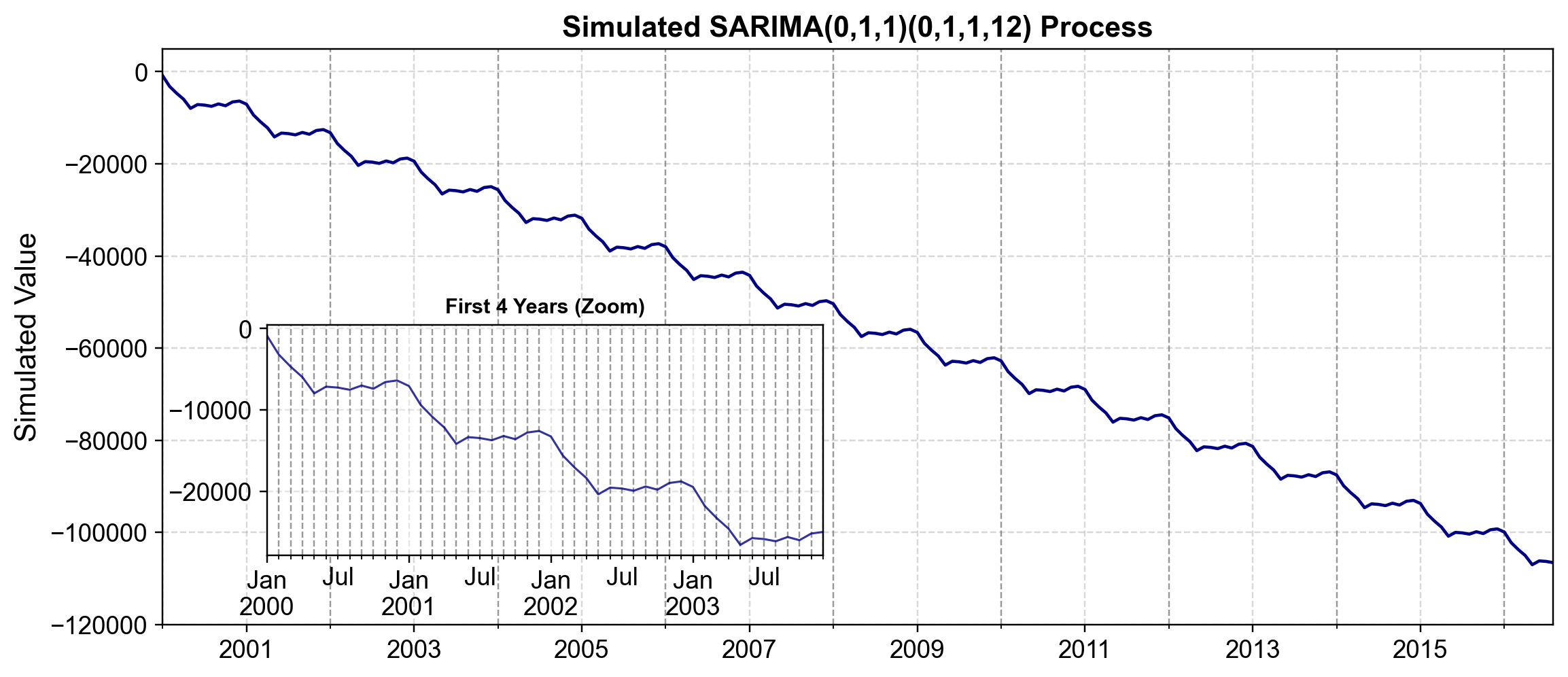
../_images/simulated_sarima_process.png — Fig. 4.23 **Simulated SARIMA(0,1,1)(0,1,1,12) Process.** The main panel displays the long-run trajectory of a synthetic monthly time series simulated from the “Airline Model” with one regular difference (\(d=1\)), one seasonal difference at period 12 (\(D=1, s=12\)), and negative moving-average parameters (\(\theta_1=-0.4, \Theta_1=-0.6\)) with innovation variance \(\sigma^2=1.0\). The simulation is generated with a fixed seed / random state (set to 42) so the same sample path is reproducible across runs. The inset panel (“First 4 Years”) zooms into the initial 48 months to emphasize the recurring within-year oscillation implied by the seasonal structure.#

Fig. 4.23 aligns with the raw simulated values (excerpted below), where the series starts at \(-856.9345\) in 2000-01-01 and is around \(-106{,}592\) by 2016-08-01. This reinforces two behaviors of the SARIMA(0,1,1)(0,1,1,12) “Airline Model” specification.

Stochastic trend (Main panel): The pronounced long-run drift arises from the cumulative effect of the regular and seasonal integration (\(d=1, D=1\)), meaning shocks can permanently shift the level rather than mean-reverting quickly.
Stable seasonality (Inset): The first 48 months show a smooth, repeating annual pattern consistent with a 12-month seasonal component, and the negative seasonal MA term (\(\Theta_1=-0.6\)) contributes to that “smooth” seasonal waveform rather than a jagged alternation.

4.6.5. SARIMAX: Modeling with External Drivers#

While SARIMA is a powerful framework, it relies solely on the history of the variable itself—for instance, predicting future sales using only past sales figures. However, real-world time series are often influenced by independent external forces:

Sales might drop due to a price hike.
Traffic might spike because of a holiday.
Inflation might jump during an energy crisis.

To capture these relationships, we extend our framework to SARIMAX (Seasonal ARIMA with eXogenous regressors).

4.6.5.1. The “Side Window” Analogy#

We can think of the difference between these models using a driving analogy:

ARIMA/SARIMA is like driving while looking only in the rear-view mirror. You navigate by assuming the road ahead will follow the same patterns (curves, bumps) as the road behind you.
SARIMAX allows you to look out the side window. If you see a storm approaching (external data), you can adjust your driving (forecast) immediately, even if the road behind you was sunny.

4.6.5.2. The Equation#

Mathematically, SARIMAX is often implemented as a “Regression with ARIMA errors.” We can think of the series \(Y_t\) as a combination of a regression on the external data and a residual error term that has its own time-dependent structure:

(4.27)#\[\begin{equation} Y_t = \underbrace{\beta X_t}_{\text{External Driver}} + \underbrace{\eta_t}_{\text{ARIMA Process}} \end{equation}\]

Where:

\(X_t\) is the external variable (or matrix of variables).
\(\beta\) captures the immediate impact of the external driver.
\(\eta_t\) is the “noise” or residual, which is not random but follows an ARIMA pattern (the “internal momentum”).

4.6.6. Example 2: Quarterly WPI (Sparse Seasonality)#

This example demonstrates how to model weak or irregular seasonality. The US Wholesale Price Index (WPI) generally follows a stable upward trend, but it contains specific shocks (like the 1973 Oil Crisis) that create echoes in the data.

Unlike the Airline passenger data, which has a rigid, dominant annual cycle, the WPI has “sparse” seasonality—shocks that repeat quarterly but don’t necessarily justify a complex multiplicative model. We use this to demonstrate how to specify custom lag polynomials in statsmodels, allowing us to target specific seasonal lags (e.g. lag 4) without forcing a full seasonal structure.

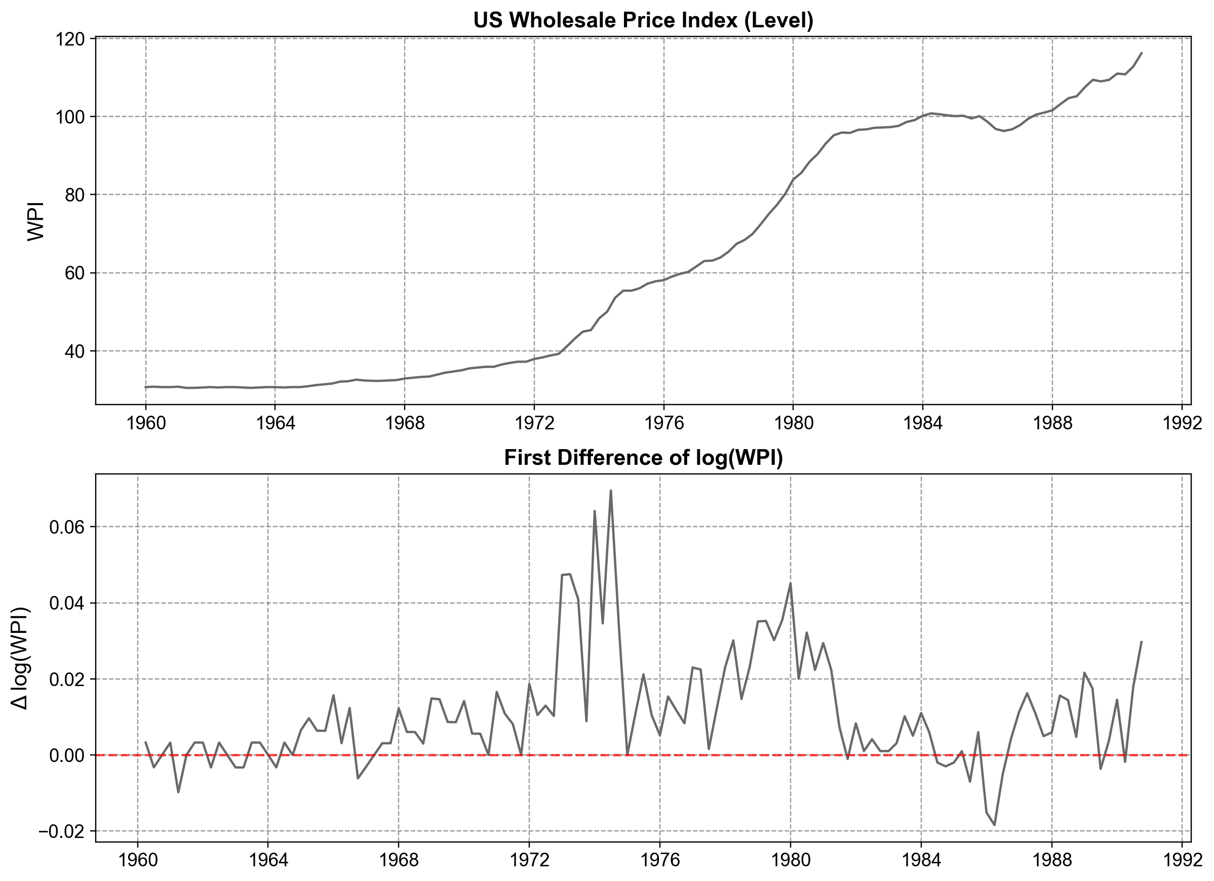
../_images/wpi_levels_differences.png — Fig. 4.24 US Wholesale Price Index (WPI) in levels (top) and first difference of log(WPI) (bottom). The level series shows a clear upward trend and changing growth rates, whereas the differenced log series fluctuates around zero with more stable variability, indicating that taking first differences of the logarithm is an effective step toward stationarity for subsequent ARIMA/SARIMA modeling.#

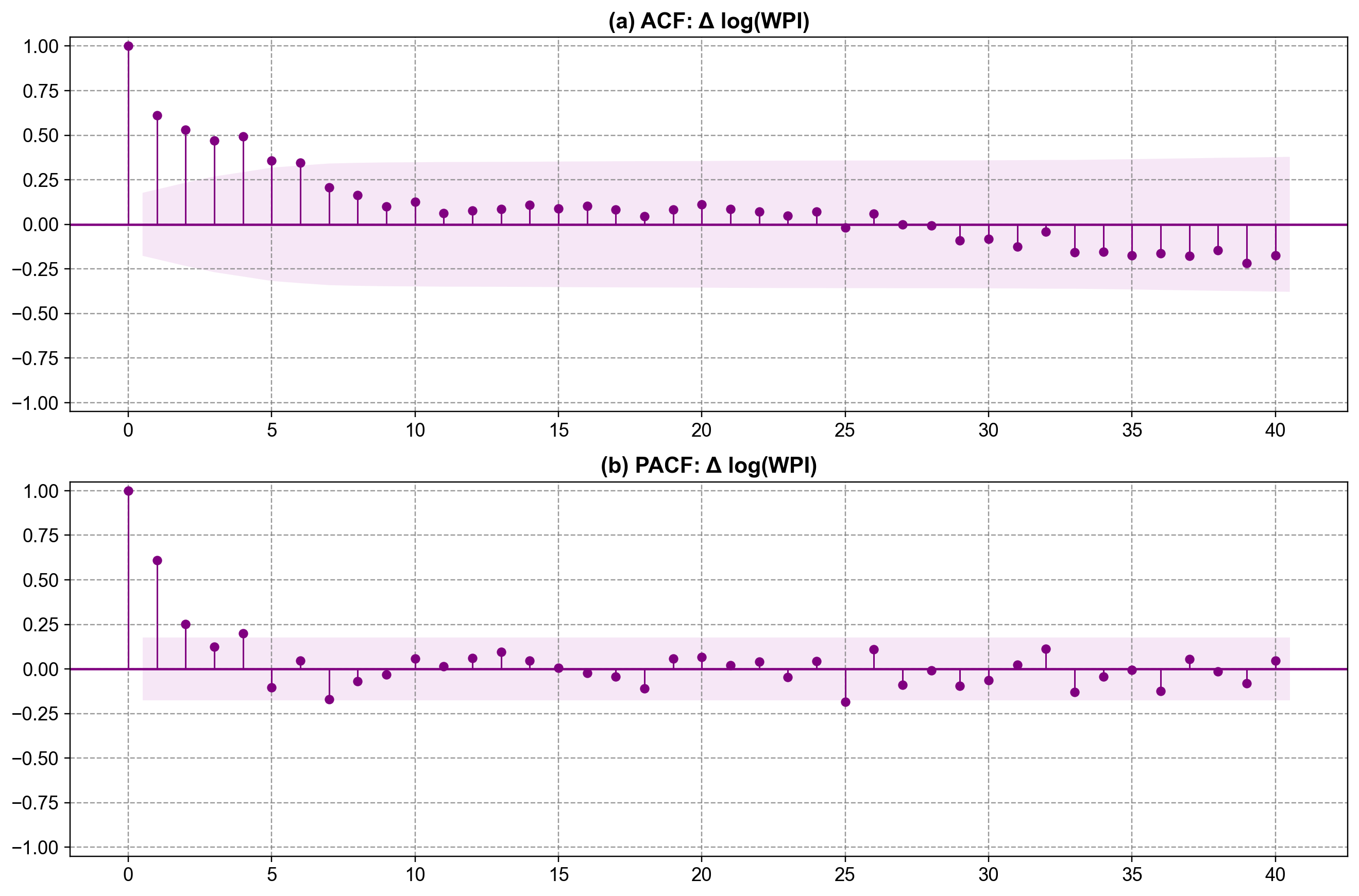
../_images/wpi_differences_acf_pacf.png — Fig. 4.25 Sample ACF and PACF of the first difference of log(WPI). Panel **(a)** shows a slowly decaying ACF with notable positive autocorrelations at the first few lags, indicating substantial short‑run persistence in growth rates. Panel **(b)** displays a PACF with a strong spike at lag 1 and smaller but still visible spikes at a few subsequent lags, a pattern compatible with a low‑order ARMA specification on the differenced log series and motivating models such as ARIMA(1,1,1) with additional structure for mild seasonal effects.#

To implement this specialized structure in [Statsmodels Developers, 2023], we define a custom Moving Average polynomial. Specifically, we want to include an MA term at lag 1 (standard smoothing) and an MA term at lag 4 (quarterly seasonality), skipping lags 2 and 3. We pass this structure as (1, 0, 0, 1):

                                 SARIMAX Results                                 
=================================================================================
Dep. Variable:                    ln_wpi   No. Observations:                  124
Model:             SARIMAX(1, 1, [1, 4])   Log Likelihood                 386.034
Date:                   Fri, 02 Jan 2026   AIC                           -762.067
Time:                           19:37:51   BIC                           -748.006
Sample:                       01-01-1960   HQIC                          -756.356
                            - 10-01-1990                                         
Covariance Type:                     opg                                         
==============================================================================
                 coef    std err          z      P>|z|      [0.025      0.975]
------------------------------------------------------------------------------
intercept      0.0024      0.002      1.488      0.137      -0.001       0.006
ar.L1          0.7801      0.095      8.250      0.000       0.595       0.965
ma.L1         -0.3987      0.126     -3.168      0.002      -0.645      -0.152
ma.L4          0.3094      0.120      2.578      0.010       0.074       0.545
sigma2         0.0001    9.8e-06     11.111      0.000    8.97e-05       0.000
===================================================================================
Ljung-Box (L1) (Q):                   0.02   Jarque-Bera (JB):                45.12
Prob(Q):                              0.90   Prob(JB):                         0.00
Heteroskedasticity (H):               2.57   Skew:                             0.29
Prob(H) (two-sided):                  0.00   Kurtosis:                         5.91
===================================================================================

Warnings:
[1] Covariance matrix calculated using the outer product of gradients (complex-step).

This model successfully captures the data’s structure by combining:

One regular difference on \(\log(\text{WPI})\) to stabilize the trend.
Non-seasonal AR(1) and MA(1) terms for short-term dynamics.
An additive seasonal MA(4) term to capture the quarterly cycle.

This approach—using sparse lag polynomials—is a useful stepping stone between pure ARIMA and the fully multiplicative SARIMA models we discuss next.

4.6.7. Example 3: Airline Data (Multiplicative Seasonality)#

This example demonstrates the canonical multiplicative SARIMA model. The Airline dataset tracks monthly passenger counts and is famous for its strong, stable, and evolving seasonal pattern.

Unlike the WPI data, where seasonality was “additive” and sparse, the Airline data requires a multiplicative structure. The seasonal pattern (travel peaks in summer) grows in magnitude as the overall trend increases. This makes it the perfect dataset to introduce the full SARIMA specification \((p,d,q) \times (P,D,Q)_{12}\), where the seasonal component multiplies the non-seasonal component.

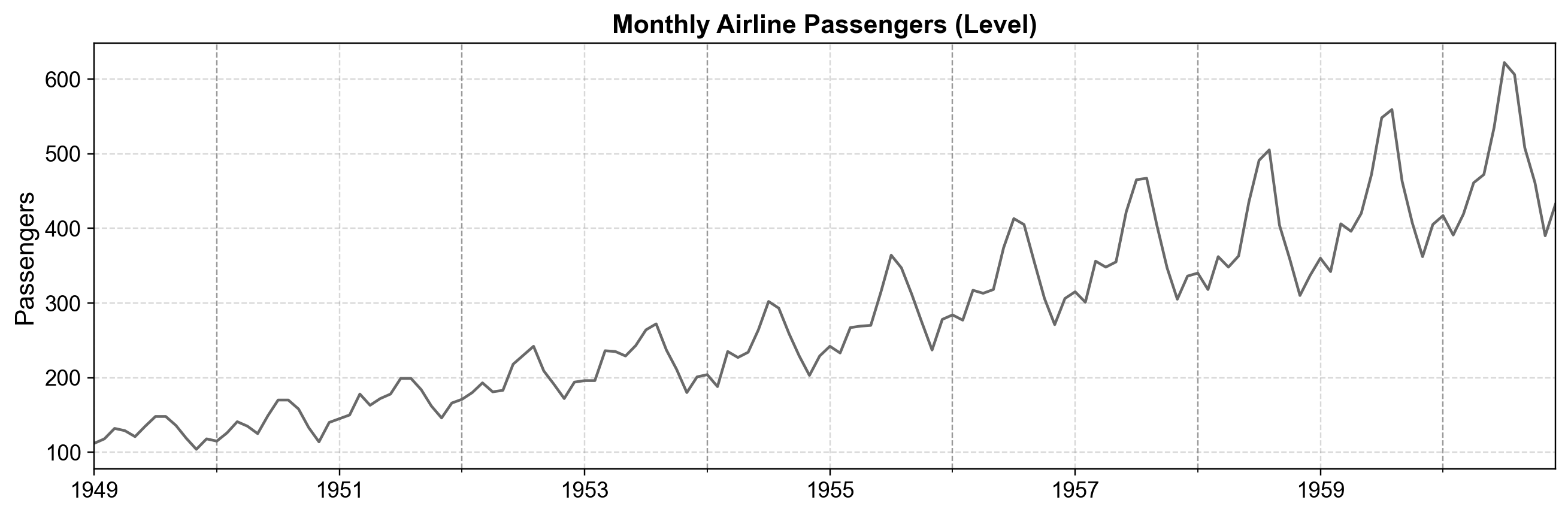
../_images/airline_passengers_level.png — Fig. 4.26 Monthly international airline passengers from 1949 to 1960 (level series). The plot displays a strong upward trend and pronounced annual seasonality, with peaks increasing over time—a classic example used to illustrate multiplicative SARIMA models.#

We specify a SARIMA(2,1,0)×(1,1,0)\(_{12}\) model. In statsmodels, this translates to:

order=(2, 1, 0): An ARIMA(2,1,0) structure for the non-seasonal dynamics.
seasonal_order=(1, 1, 0, 12): A seasonal AR(1) term and one seasonal difference at lag 12.
simple_differencing=True: This ensures the data is explicitly differenced prior to estimation, improving compatibility with other statistical software like Stata.

                                     SARIMAX Results                                      
==========================================================================================
Dep. Variable:              D.DS12.ln(passengers)   No. Observations:                  131
Model:             SARIMAX(2, 0, 0)x(1, 0, 0, 12)   Log Likelihood                 240.821
Date:                            Fri, 02 Jan 2026   AIC                           -473.643
Time:                                    19:38:09   BIC                           -462.142
Sample:                                02-28-1950   HQIC                          -468.970
                                     - 12-31-1960                                         
Covariance Type:                              opg                                         
==============================================================================
                 coef    std err          z      P>|z|      [0.025      0.975]
------------------------------------------------------------------------------
ar.L1         -0.4057      0.080     -5.045      0.000      -0.563      -0.248
ar.L2         -0.0799      0.099     -0.809      0.419      -0.274       0.114
ar.S.L12      -0.4723      0.072     -6.592      0.000      -0.613      -0.332
sigma2         0.0014      0.000      8.403      0.000       0.001       0.002
===================================================================================
Ljung-Box (L1) (Q):                   0.01   Jarque-Bera (JB):                 0.72
Prob(Q):                              0.91   Prob(JB):                         0.70
Heteroskedasticity (H):               0.54   Skew:                             0.14
Prob(H) (two-sided):                  0.04   Kurtosis:                         3.23
===================================================================================

Warnings:
[1] Covariance matrix calculated using the outer product of gradients (complex-step).

The summary table confirms that the seasonal AR term (ar.S.L12) is statistically significant, validating the presence of strong annual dependence even after differencing.

4.6.8. Example 4: Friedman Consumption (Exogenous Regressors)#

This example demonstrates the true power of SARIMAX by including an external variable. We use the Friedman consumption dataset, which tracks US personal consumption.

Forecasting consumption based solely on its own history is limited because consumption is heavily driven by economic policy. By including Money Supply (M2) as an exogenous regressor (\(X_t\)), we can test if information from the broader economy improves our ability to predict consumption (\(Y_t\)). This example also serves to illustrate the critical difference between one-step-ahead and dynamic forecasting.

4.6.8.1. Dynamic Forecasting with SARIMAX#

In many applications, we require multi‑step forecasts where predictions rely on previous forecasts rather than observed data. To illustrate the difference between one-step-ahead and dynamic forecasting, we utilize the Friedman consumption dataset. Here, we model consumption with ARMA(1,1) errors and include money supply (m2) as an exogenous regressor [Statsmodels Developers, 2023].

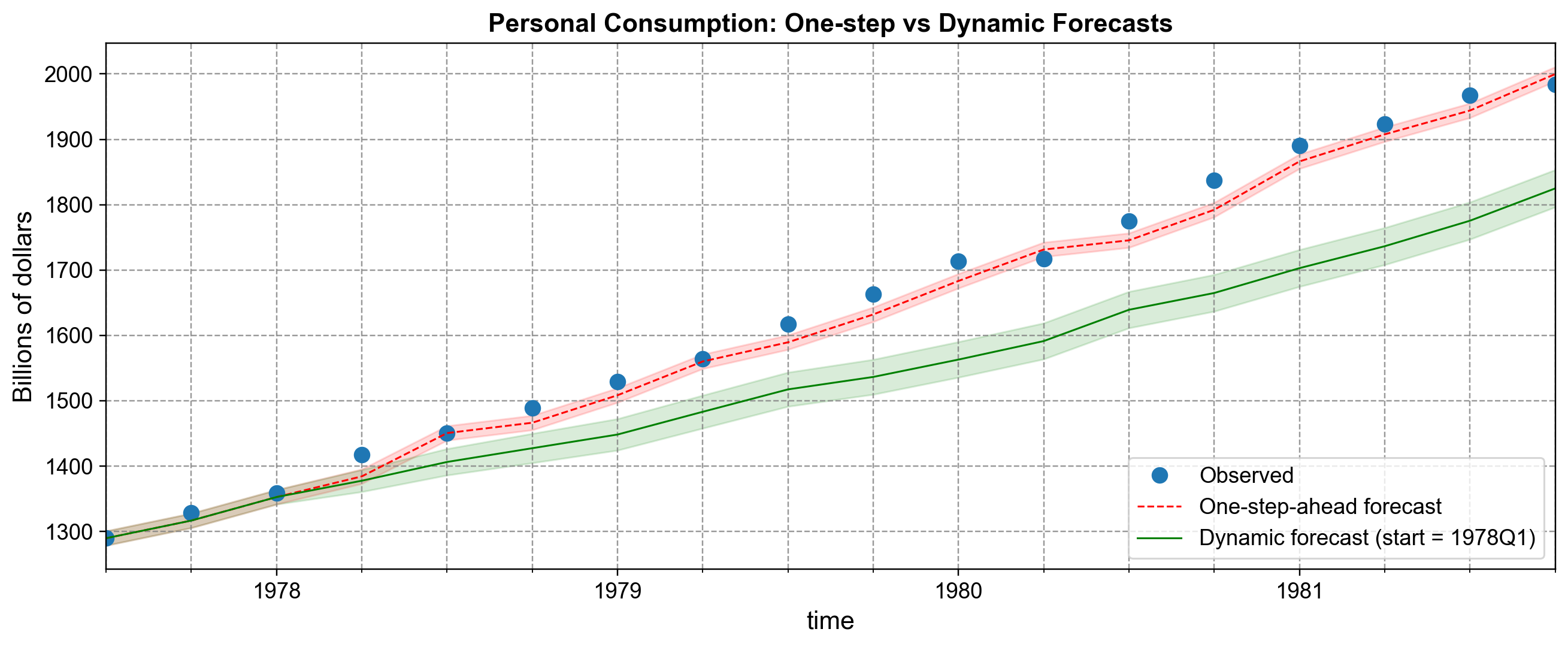
../_images/friedman_consumption_forecasts.png — Fig. 4.27 One-step-ahead and dynamic SARIMAX forecasts for quarterly US personal consumption from 1977Q3 to 1981Q4. One-step-ahead forecasts closely track the observed series, because each prediction conditions on the latest observed value of consumption, while dynamic forecasts starting in 1978Q1 gradually diverge as forecast uncertainty accumulates [Statsmodels Developers, 2023].#

In Fig. 4.27, the blue dots show the realized consumption levels, the red dashed line shows the one‑step‑ahead forecasts, and the green line shows dynamic forecasts initialized in 1978Q1. The widening shaded regions around each line are 95% prediction intervals, and they emphasize how uncertainty grows as we move further into the future under dynamic forecasting, even though we use the same underlying SARIMAX model.

4.6.8.2. Forecast Error Diagnostics#

To better understand the difference between the two forecasting strategies, we can look directly at the forecast errors, defined as “forecast − actual”, for both one‑step‑ahead and dynamic predictions. If the model is well specified, one‑step‑ahead errors should fluctuate around zero with no obvious structure, whereas dynamic forecast errors may drift as small biases accumulate across multiple steps [Statsmodels Developers, 2023].

../_images/sarimax_friedman_forecast_errors.png — Fig. 4.28 Forecast errors for one-step-ahead and dynamic SARIMAX predictions of US personal consumption. One-step-ahead errors remain close to zero and mostly within the 95% prediction bands, suggesting that the ARMA(1,1) error structure captures short-run dependence well, whereas dynamic forecast errors become increasingly negative over time, illustrating how multi-step forecasting can accentuate small model misspecification or bias [Statsmodels Developers, 2023].#

We see that the one‑step‑ahead errors (blue) remain relatively small and centered near zero, which is what we expect from a reasonably well‑fitting model. In contrast, the dynamic forecast errors (red) drift downward as the horizon extends, demonstrating that using previous forecasts as inputs can introduce systematic deviations when the model is even slightly mis‑specified or when shocks accumulate over time.