Remark

Please be aware that these lecture notes are accessible online in an ‘early access’ format. They are actively being developed, and certain sections will be further enriched to provide a comprehensive understanding of the subject matter.

1.3. Time Series Cross-Validation

1.3.1. Cross-Validation

Cross-validation is a powerful statistical technique used in machine learning for model selection and performance evaluation. It is particularly useful for smaller datasets and helps ensure that models generalize well to unseen data. By systematically partitioning the data into subsets for training and validation, cross-validation provides a more robust assessment of model performance than simple train-test splits [James et al., 2023].

Purpose and Benefits

1. Model Selection:

   • Helps choose the best model or hyperparameters for a given task.

   • Allows comparison of different models or algorithms on the same data.

   • Provides a systematic way to tune hyperparameters for optimal performance [Refaeilzadeh et al., 2009].

2. Performance Estimation:

   • Provides a more reliable estimate of model performance on unseen data.

   • Reduces the impact of data partitioning luck by using multiple train-test splits.

   • Offers insights into the model’s stability and sensitivity to data variations [James et al., 2023].

3. Overfitting Prevention:

   • Reduces the risk of overfitting by using multiple subsets of data for training and validation.

   • Helps identify models that are too complex or too simple for the given data.

   • Encourages the development of more generalizable models [Refaeilzadeh et al., 2009].

1.3.2. Why Standard Cross-Validation Fails for Time Series

Traditional k-fold cross-validation randomly partitions data into folds, which violates the temporal structure of time series data. This can lead to:

• Data leakage: Using future information to predict past events

• Unrealistic performance estimates: Models appear more accurate than they would be in practice

• Violation of temporal dependencies: Breaking the sequential nature that drives time series patterns

Example: If we randomly split stock price data, we might train on 2023 data and test on 2021 data, which is impossible in real forecasting scenarios.

1.3.3. Time Series Cross-Validation

Time Series Cross-Validation is a specialized technique designed for evaluating models on time-dependent data. This method is crucial for maintaining the chronological order of observations, which is essential in time series analysis. Here’s an expanded explanation:

1. Sliding Window Approach:

   • Uses a forward-moving time window for training and testing.

   • The training set grows with each iteration, while the test set remains a fixed size.

   • This approach mimics real-world forecasting scenarios where we use past data to predict future values.

2. Maintaining Temporal Order:

   • Preserves the time-based dependencies in the data.

   • Ensures that future information is not used to predict past events, avoiding data leakage.

3. Multiple Train-Test Splits:

   • Creates several train-test splits, each representing a different point in time.

   • Allows for assessing model performance across various temporal segments of the data.

4. Forecasting Performance Assessment:

   • Evaluates how well the model generalizes to future, unseen data.

   • Particularly useful for assessing the stability of model performance over time.

5. Adaptability to Changing Patterns:

   • Helps in understanding how model performance might change as new data becomes available.

   • Useful for detecting concept drift in time series.

6. Fixed Window (Rolling Origin):

   • Training window size remains constant as it moves forward

   • Useful when recent patterns are more relevant than distant history

   • Example: Always use exactly 252 trading days (1 year) for training

7. Expanding Window (Used in our example):

   • Training window grows with each split

   • Incorporates all available historical information

   • Better for capturing long-term trends and structural changes

8. Blocked Cross-Validation:

   • Introduces gaps between training and test sets

   • Accounts for temporal correlation that might persist beyond immediate neighbors

   • Useful when autocorrelation extends over multiple periods

Example using NVIDIA (NVDA) stock price data:

Show code cell source

Hide code cell source

import yfinance as yf
# Download NVIDIA stock data
data = yf.download(['NVDA'], period='5y', progress=False, auto_adjust=True)
data = data['Close'].reset_index()

Loading ITables v2.5.2 from the init_notebook_mode cell... (need help?)

1.3.4. Types of Time Series Cross-Validation

The three main approaches to time series cross-validation differ fundamentally in how they handle training data over time. The timeline visualization below illustrates the key distinctions between expanding window, rolling window, and blocked cross-validation methods:

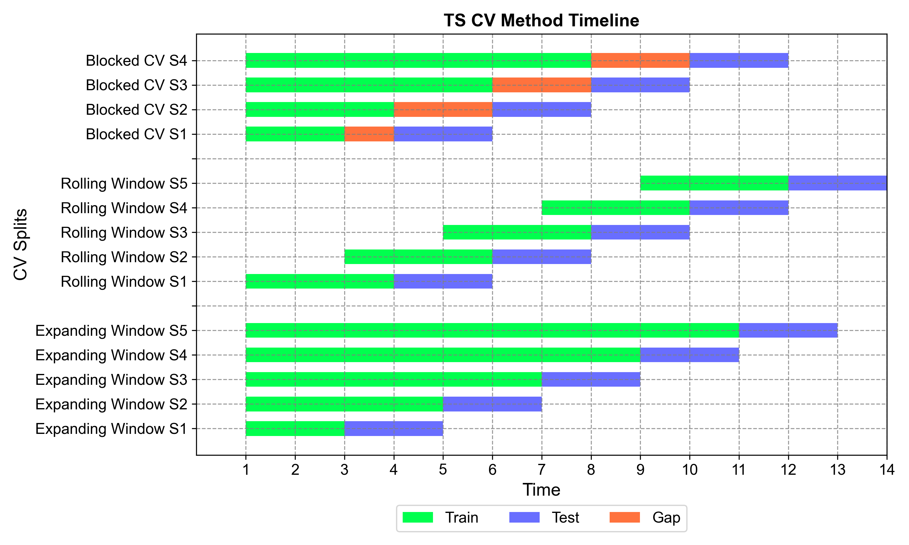
Fig. 1.2 Timeline comparison of three time series cross-validation methods. The visualization shows how each method handles training data (green), test data (blue), and gaps (orange) across multiple splits over time. Expanding window grows training sets progressively, rolling window maintains fixed training sizes, and blocked CV introduces purged gaps to prevent data leakage.

Method Comparison Overview:

Expanding Window Cross-Validation (Top section):

• Training sets grow progressively with each split, accumulating all historical data

• Maximizes available information for model training

• Best for capturing long-term trends and when all historical context is valuable

• Each split builds upon all previous knowledge, creating increasingly comprehensive training sets

Rolling Window Cross-Validation (Middle section):

• Fixed training window size that slides forward through time

• Maintains consistent training periods (e.g., always 200 days)

• Emphasizes recent patterns while discarding older information

• Ideal for non-stationary series where recent data is more predictive than distant history

Blocked Cross-Validation (Bottom section):

• Introduces purged gaps (orange) between training and test periods

• Prevents data leakage from autocorrelation and temporal dependencies

• Training sets expand but stop before test periods with buffer zones

• Essential for financial data and high-frequency time series with strong serial correlation

Key Temporal Insights:

The timeline clearly shows how each method treats the temporal boundary between training and testing:

• Expanding: Direct transition from training to testing (no gaps)

• Rolling: Direct transition but with limited historical memory

• Blocked: Intentional gaps to break temporal correlations

Selection Criteria:

• Choose Expanding Window for trend-following models and when historical patterns remain relevant

• Select Rolling Window for adaptive models in changing environments with structural breaks

• Use Blocked CV when autocorrelation is present and realistic performance estimates are critical

Each method serves different analytical needs and data characteristics, making the choice dependent on your specific time series properties and forecasting objectives.

1.3.4.1. Expanding Window

The Expanding Window approach (also known as “growing window” or “anchored walk-forward”) is the default method in scikit-learn’s TimeSeriesSplit. This technique progressively increases the training window size while maintaining consistent test set sizes, making it particularly valuable for capturing evolving patterns in time series data.

Key Characteristics

Progressive Data Accumulation: Each subsequent split incorporates all previous training data plus additional historical observations, creating an ever-expanding knowledge base for the model. This cumulative approach ensures that valuable historical patterns and long-term trends are preserved across all validation splits.

Mimicking Real-World Scenarios: In practice, analysts and traders typically have access to all historical data when making forecasts. The expanding window method closely replicates this reality, where decision-makers use the entirety of available historical information rather than discarding older data.

Long-term Pattern Recognition: By retaining all historical data, this method is particularly effective at capturing:

• Structural changes that occur gradually over time

• Long-term cycles and secular trends

• Regime changes in market conditions or business environments

• Seasonal patterns that may evolve or strengthen over time

When to Use Expanding Windows

• Sufficient Historical Data: When you have adequate historical observations to support meaningful training

• Evolving Relationships: When relationships between variables may strengthen or change over time

• Long-term Dependencies: For time series where distant past observations remain relevant

• Model Stability Testing: To assess how model performance changes as more data becomes available

Trade-offs to Consider:

• Computational Cost: Training time increases with each split as the training set grows

• Concept Drift: May be less responsive to recent structural changes if older patterns dominate

• Memory Requirements: Larger training sets require more computational resources

The NVIDIA example below demonstrates these concepts in action, showing how each split builds upon previous knowledge while testing the model’s ability to generalize to future periods.

Show code cell source

Hide code cell source

from sklearn.model_selection import TimeSeriesSplit

# Time Series Cross-Validation
tscv = TimeSeriesSplit(n_splits=5)

for i, (train_index, test_index) in enumerate(tscv.split(data),1):
      # Display split periods
    print('\033[1;31m' + f'Split {i}:' + '\033[0m')
    print("\t\033[1;42mTrain set\033[0m:", f'\t\tFrom {data.loc[train_index.min(), "Date"].strftime("%Y-%m-%d")} '
          f'To {data.loc[train_index.max(), "Date"].strftime("%Y-%m-%d")}')
    print("\t\033[1;44mTest set\033[0m:", f'\t\tFrom {data.loc[test_index.min(), "Date"].strftime("%Y-%m-%d")} '
          f'To {data.loc[test_index.max(), "Date"].strftime("%Y-%m-%d")}')

Split 1:
	Train set: 		From 2020-11-30 To 2021-09-30
	Test set: 		From 2021-10-01 To 2022-08-01
Split 2:
	Train set: 		From 2020-11-30 To 2022-08-01
	Test set: 		From 2022-08-02 To 2023-05-31
Split 3:
	Train set: 		From 2020-11-30 To 2023-05-31
	Test set: 		From 2023-06-01 To 2024-04-01
Split 4:
	Train set: 		From 2020-11-30 To 2024-04-01
	Test set: 		From 2024-04-02 To 2025-01-30
Split 5:
	Train set: 		From 2020-11-30 To 2025-01-30
	Test set: 		From 2025-01-31 To 2025-11-28

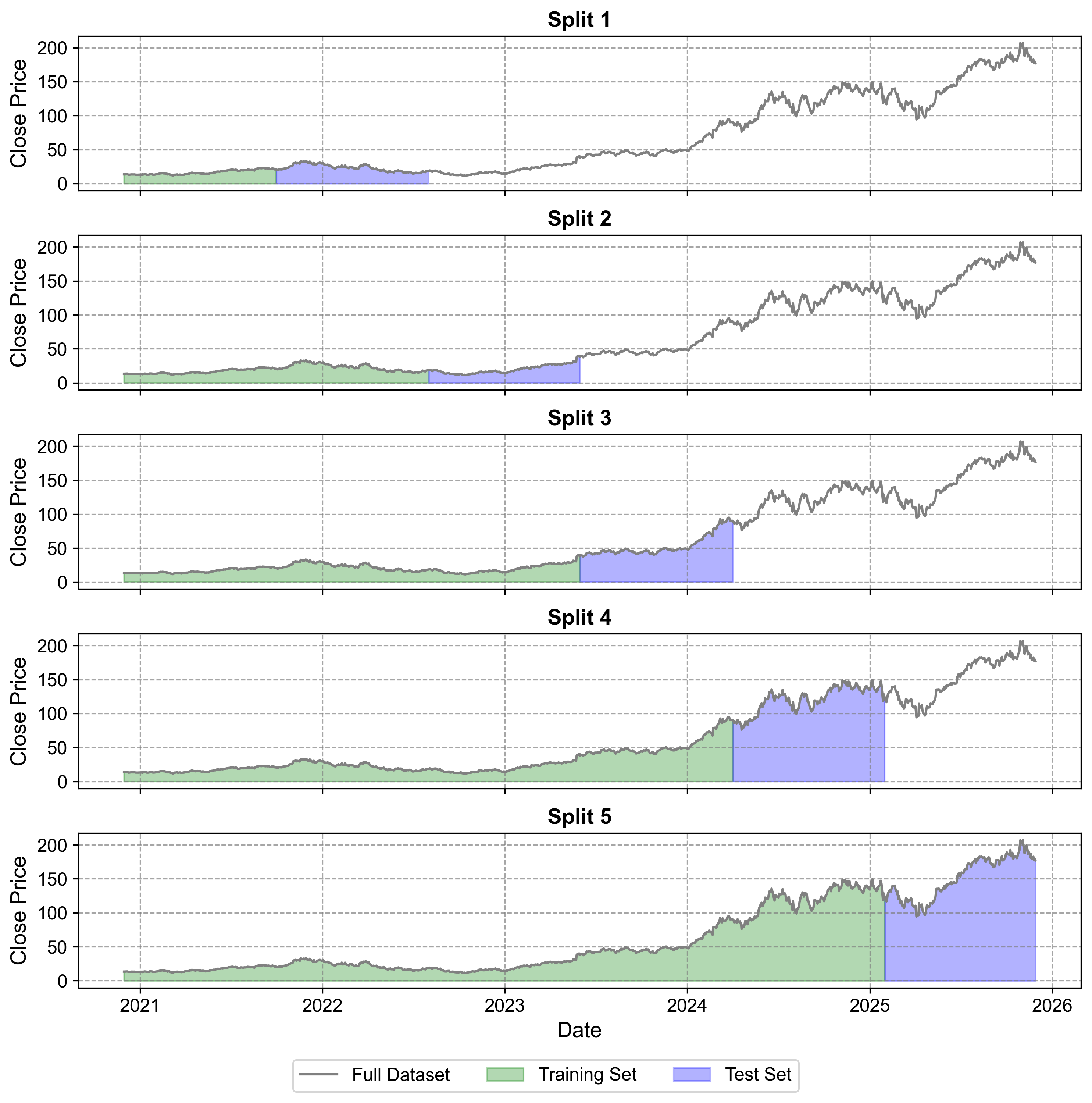
Fig. 1.3 Time Series Cross-Validation splits for NVIDIA stock price data (2020-2025). The visualization shows five sequential splits with expanding training windows (green) and fixed-size test sets (blue). Each split demonstrates the forward-moving nature of the validation process, with the gray line representing the complete dataset. The stock price shows significant growth, particularly in 2023-2025, ranging from around $0 to $150.

Split Structure

• Each split shows:

  • Training data (green shaded area)

  • Test data (blue shaded area)

  • Full dataset line (gray)

• The training window expands with each subsequent split

• Test set size remains consistent across all splits

Progressive Nature

• Split 1: Uses minimal training data with early test period

• Split 2: Expands training data forward

• Split 3: Further expansion of training window

• Split 4: Includes significant price increase period

• Split 5: Uses maximum training data, testing on most recent period

1.3.4.2. Rolling/Sliding Window Cross-Validation

Definition: Rolling Window Cross-Validation (also known as Fixed Window or Sliding Window) maintains a constant training window size that slides forward with each split, emphasizing recent data patterns over historical information.

Key Characteristics:

• Training window size remains fixed as it moves forward

• Useful when recent patterns are more relevant than distant history

• Also called “Rolling Origin” validation

• Preferable when older history may not be relevant due to structural changes

When to Use:

• Large datasets with sufficient observations

• When structural changes occur over time (e.g., market regime shifts)

• When you want to simulate real-world scenarios where only recent data is available

• Example: Using exactly 252 trading days (1 year) for training, always

Show code cell content

Hide code cell content

from sklearn.model_selection import TimeSeriesSplit
import numpy as np

# Custom Rolling Window implementation
class RollingTimeSeriesSplit:
    def __init__(self, n_splits=5, train_size=None, test_size=None):
        self.n_splits = n_splits
        self.train_size = train_size
        self.test_size = test_size
    
    def split(self, X):
        n_samples = len(X)
        if self.test_size is None:
            test_size = n_samples // (self.n_splits + 1)
        else:
            test_size = self.test_size
            
        if self.train_size is None:
            train_size = test_size * 2  # Default: 2x test size
        else:
            train_size = self.train_size
        
        for i in range(self.n_splits):
            start_train = i * test_size
            end_train = start_train + train_size
            start_test = end_train
            end_test = start_test + test_size
            
            if end_test <= n_samples:
                train_indices = np.arange(start_train, end_train)
                test_indices = np.arange(start_test, end_test)
                yield train_indices, test_indices

# Example usage with NVIDIA data
rolling_cv = RollingTimeSeriesSplit(n_splits=4, train_size=200, test_size=50)

print("Rolling Window Cross-Validation:")
for i, (train_idx, test_idx) in enumerate(rolling_cv.split(data), 1):
    print(f"Split {i}:")
    print(f"\tTrain: From {data.loc[train_idx.min(), 'Date'].strftime('%Y-%m-%d')} "
          f"To {data.loc[train_idx.max(), 'Date'].strftime('%Y-%m-%d')} "
          f"({len(train_idx)} days)")
    print(f"\tTest: From {data.loc[test_idx.min(), 'Date'].strftime('%Y-%m-%d')} "
          f"To {data.loc[test_idx.max(), 'Date'].strftime('%Y-%m-%d')} "
          f"({len(test_idx)} days)")

Rolling Window Cross-Validation:
Split 1:
	Train: From 2020-11-30 To 2021-09-15 (200 days)
	Test: From 2021-09-16 To 2021-11-24 (50 days)
Split 2:
	Train: From 2021-02-11 To 2021-11-24 (200 days)
	Test: From 2021-11-26 To 2022-02-07 (50 days)
Split 3:
	Train: From 2021-04-26 To 2022-02-07 (200 days)
	Test: From 2022-02-08 To 2022-04-20 (50 days)
Split 4:
	Train: From 2021-07-07 To 2022-04-20 (200 days)
	Test: From 2022-04-21 To 2022-07-01 (50 days)

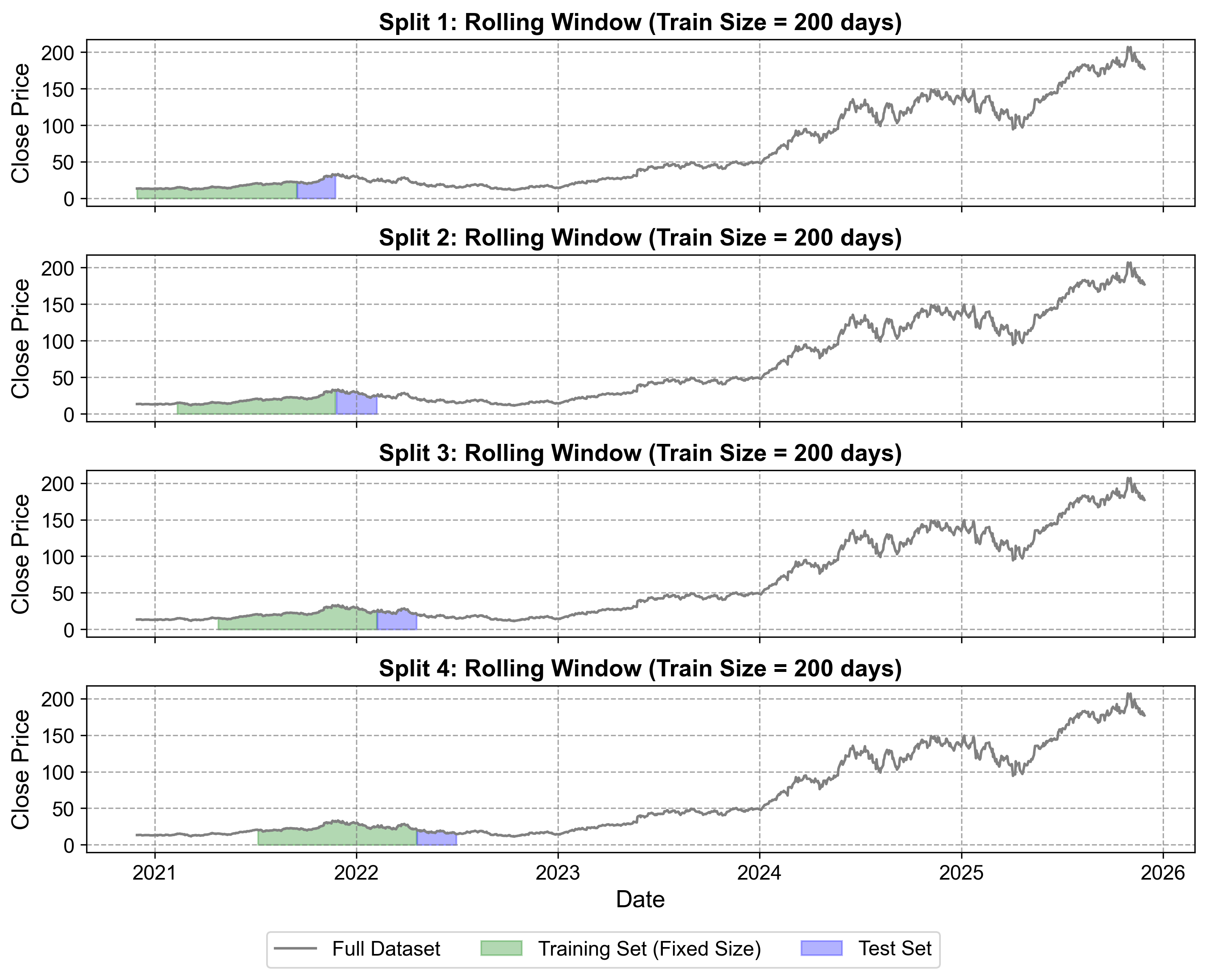
Fig. 1.4 Rolling Window Cross-Validation for NVIDIA stock price data (2020-2022). The visualization demonstrates four sequential splits with fixed-size training windows (green) that slide forward through time, maintaining consistent 200-day training periods. Unlike expanding windows, each training set discards older data as it moves forward, focusing on the most recent 200 days of market behavior. Test sets (blue) remain consistent at 50 days each. This approach is particularly effective for capturing evolving market dynamics during NVIDIA’s transition period from gaming-focused to AI-infrastructure company.

Split Structure Comparison with Expanding Window:

• Training Data: Green shaded areas maintain constant size (200 days each), sliding forward through time

• Data Focus: Each split emphasizes recent patterns by discarding older historical data

• Temporal Progression: Windows move forward systematically, maintaining the same “memory length”

Key Observations from Rolling Window Method:

Rolling Window Advantages Demonstrated:

• Adaptability: Each model focuses on the most recent 200-day pattern, quickly adapting to new market conditions

• Structural Change Detection: Better captures the evolving nature of NVIDIA’s business model transformation

• Reduced Historical Bias: Avoids influence from outdated market patterns (e.g., pre-AI era pricing)

• Consistent Memory: All models use identical training periods, enabling fair performance comparisons

Market Context Analysis:

• Early Splits: Focus on gaming and cryptocurrency mining demand cycles

• Later Splits: Begin incorporating early AI/data center growth signals

• Pattern Evolution: Shows how rolling windows capture the company’s strategic pivot more dynamically than expanding windows

Advantages:

• Adapts to new data trends through the rolling mechanism

• Provides more robust forecasts in dynamic environments

• Prevents overfitting through consistent window size

• Better for non-stationary time series with structural breaks

Disadvantages:

• May discard valuable historical information

• Requires sufficient data for meaningful window sizes

• Less suitable for capturing long-term patterns

1.3.4.3. Blocked Cross-Validation

Definition: Blocked Cross-Validation introduces gaps (blocking periods) between training and test sets to reduce temporal correlation and minimize data leakage due to autocorrelation.

Key Concepts:

1. Purging: Eliminates observations from the training set that have labels overlapping in time with the test set

2. Embargo: Adds an additional buffer period after the test set to eliminate serial correlation between consecutive periods

Why It’s Needed:

• Time series data exhibits autocorrelation - observations close in time are correlated

• Even without direct data leakage, temporal dependencies can leak future information into training

• Traditional CV methods can underestimate prediction errors due to these dependencies

Show code cell source

Hide code cell source

import pandas as pd
import numpy as np
from typing import Iterator, Tuple

class PurgedTimeSeriesSplit:
    def __init__(self, n_splits: int = 5, embargo_pct: float = 0.05, 
                 purge_pct: float = 0.02):
        """
        Purged Time Series Cross-Validation with embargo
        
        Parameters:
        -----------
        n_splits : int
            Number of splits
        embargo_pct : float
            Percentage of data to embargo after test set
        purge_pct : float  
            Percentage of data to purge before test set
        """
        self.n_splits = n_splits
        self.embargo_pct = embargo_pct
        self.purge_pct = purge_pct
    
    def split(self, X: pd.DataFrame) -> Iterator[Tuple[np.ndarray, np.ndarray]]:
        n_samples = len(X)
        test_size = n_samples // (self.n_splits + 1)
        
        # Calculate embargo and purge sizes
        embargo_size = int(n_samples * self.embargo_pct)
        purge_size = int(n_samples * self.purge_pct)
        
        for i in range(self.n_splits):
            # Test set boundaries
            test_start = (i + 1) * test_size
            test_end = test_start + test_size
            
            if test_end >= n_samples:
                break
                
            # Training set (before test set, with purging)
            train_end = test_start - purge_size
            train_indices = np.arange(0, max(0, train_end))
            
            # Test set
            test_indices = np.arange(test_start, test_end)
            
            # Apply embargo: exclude period after test set from next training
            # (This affects subsequent iterations)
            
            yield train_indices, test_indices

# Example usage
purged_cv = PurgedTimeSeriesSplit(n_splits=4, embargo_pct=0.05, purge_pct=0.02)

print("Blocked/Purged Cross-Validation:")
for i, (train_idx, test_idx) in enumerate(purged_cv.split(data), 1):
    if len(train_idx) > 0 and len(test_idx) > 0:
        # Split header
        print('\033[1;31m' + f'Split {i}:' + '\033[0m')

        # Train set (green background)
        print(
            "\t\033[1;42mTrain set\033[0m:"
            f"\tFrom {data.loc[train_idx.min(), 'Date'].strftime('%Y-%m-%d')} "
            f"To {data.loc[train_idx.max(), 'Date'].strftime('%Y-%m-%d')} "
            f"({len(train_idx)} days)"
        )

        # Test set (blue background)
        print(
            "\t\033[1;44mTest set\033[0m:"
            f"\tFrom {data.loc[test_idx.min(), 'Date'].strftime('%Y-%m-%d')} "
            f"To {data.loc[test_idx.max(), 'Date'].strftime('%Y-%m-%d')} "
            f"({len(test_idx)} days)"
        )

        # Gap (optional magenta background if you want to highlight purged days)
        gap_days = test_idx.min() - train_idx.max() - 1
        if gap_days > 0:
            print(
                "\t\033[1;45mGap\033[0m:"
                f"\t\t{gap_days} days (purged)"
            )

Blocked/Purged Cross-Validation:
Split 1:
	Train set:	From 2020-11-30 To 2021-10-21 (226 days)
	Test set:	From 2021-11-29 To 2022-11-25 (251 days)
	Gap:		25 days (purged)
Split 2:
	Train set:	From 2020-11-30 To 2022-10-20 (477 days)
	Test set:	From 2022-11-28 To 2023-11-27 (251 days)
	Gap:		25 days (purged)
Split 3:
	Train set:	From 2020-11-30 To 2023-10-20 (728 days)
	Test set:	From 2023-11-28 To 2024-11-25 (251 days)
	Gap:		25 days (purged)
Split 4:
	Train set:	From 2020-11-30 To 2024-10-21 (979 days)
	Test set:	From 2024-11-26 To 2025-11-26 (251 days)
	Gap:		25 days (purged)

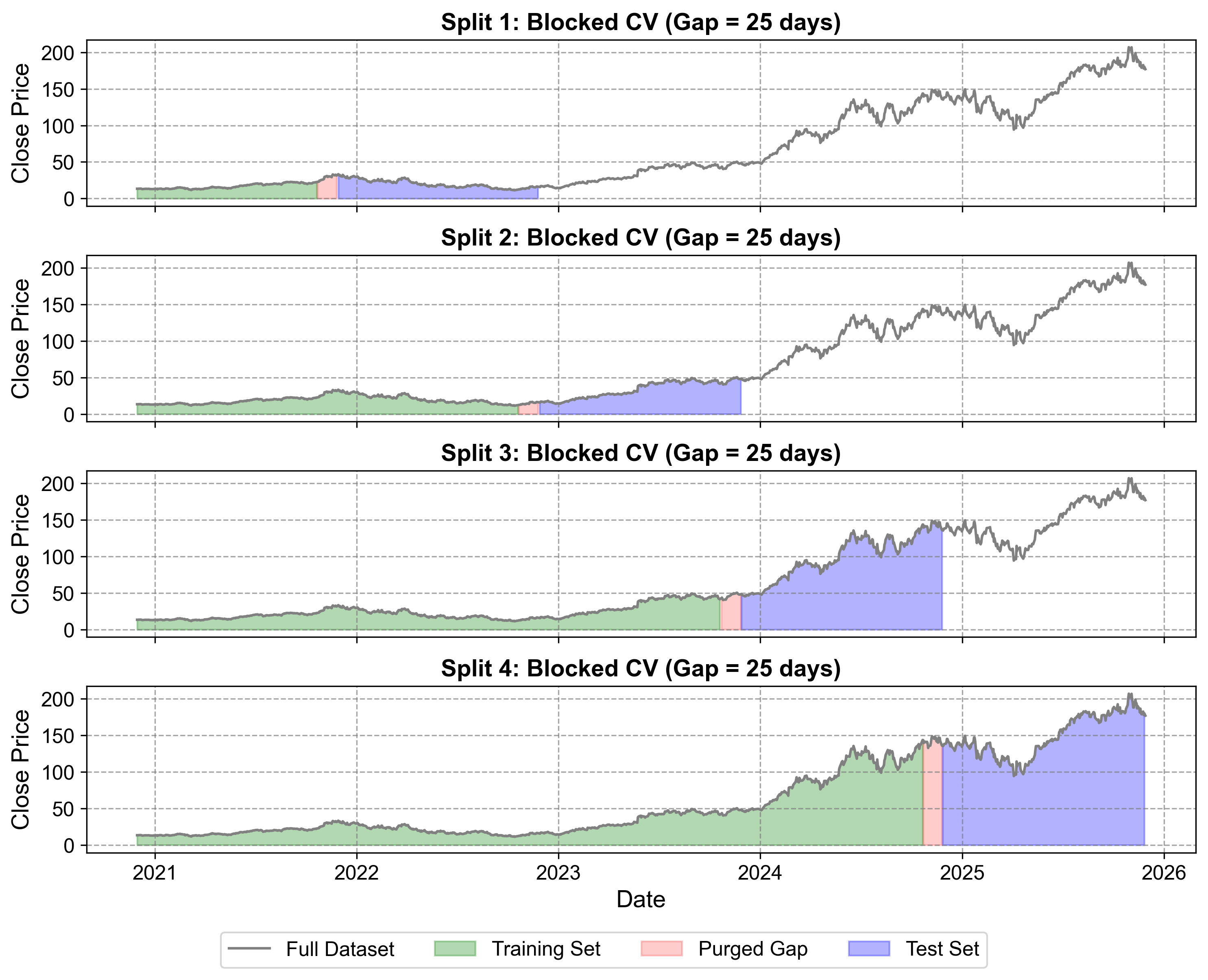
Fig. 1.5 Blocked (Purged) Cross-Validation for NVIDIA stock price data (2020-2025). This visualization demonstrates the critical concept of temporal gaps in time series validation. Training sets (green) grow over time but are separated from test sets (blue) by purged gaps (red) that prevent data leakage from autocorrelation. The 25-day gaps ensure that temporal dependencies between consecutive observations don’t artificially inflate model performance estimates. This method provides more realistic performance estimates for financial time series where price movements exhibit strong serial correlation.

Critical Features of Blocked Cross-Validation Visualization:

Purged Gaps (Red Areas):

• 25-day buffer zones between training and test sets

• Explicitly removed from both training and testing to break autocorrelation chains

• Prevent information leakage from temporally correlated observations

• Size determined by autocorrelation analysis (2% of total data in this example)

Expanding Training with Gaps:

• Training sets (green) still grow over time like expanding window CV

• But critically stop before test periods to maintain temporal independence

• Each split incorporates more historical knowledge while respecting temporal boundaries

Realistic Performance Assessment:

• Split 1: Tests model on 2021-2022 data using only pre-gap 2020-2021 training

• Split 2: Tests on 2022-2023 period with expanded training up to mid-2022 gap

• Split 3: Evaluates 2023-2024 AI boom period with comprehensive pre-2023 training

• Split 4: Tests most recent period (2024-2025) with maximum historical context

Applications:

• Financial Time Series: Where price movements exhibit strong autocorrelation

• High-frequency Data: Where serial correlation extends over multiple periods

• Label Overlap: When features are constructed using forward-looking windows

• Regulatory Compliance: When avoiding look-ahead bias is critical

Benefits:

• More accurate error estimates than standard CV

• Reduces data leakage from temporal dependencies

• Better model selection in presence of autocorrelation

• Provides more conservative (realistic) performance estimates

Practical Considerations:

• Gap Size: Should be based on autocorrelation function analysis

• Embargo Period: Typically 5-10% of total sample size

• Trade-off: Larger gaps provide better independence but reduce training data

• Computational Cost: More complex than standard CV but essential for time series

1.3.5. Practical Considerations for Time Series CV

1. Choosing the Number of Splits:

   • More splits provide better performance estimates but increase computational cost

   • Consider the trade-off between statistical reliability and practical constraints

   • Typically 3-10 splits depending on dataset size and computational resources

2. Test Set Size:

   • Should reflect the actual forecasting horizon of interest

   • For daily data: 30-90 days for monthly forecasting, 252 days for annual

   • Balance between having enough test data for reliable evaluation and sufficient training data

3. Temporal Alignment:

   • Ensure splits align with natural time boundaries (e.g., month/quarter ends for business data)

   • Consider seasonal patterns when determining split points

   • Account for calendar effects (holidays, weekends) in financial data