Seasonal-Trend Decomposition using LOESS (STL)

3.2. Seasonal-Trend Decomposition using LOESS (STL)#

3.2.1. Introduction#

Seasonal-Trend decomposition using LOESS (STL) is a powerful and versatile statistical method for decomposing time series data into three fundamental components: trend, seasonal, and residual (remainder). Developed by Cleveland, Cleveland, McRae, and Terpenning in their seminal 1990 paper published in the Journal of Official Statistics, STL has become one of the most widely used decomposition techniques in time series analysis [Cleveland et al., 1990].

The method leverages LOESS (Locally Estimated Scatterplot Smoothing), also known as LOWESS (Locally Weighted Scatterplot Smoothing), to extract smooth estimates of each component. This approach combines the simplicity of linear regression with the flexibility of nonlinear modeling, making it particularly effective for real-world data that exhibits complex patterns.

3.2.1.1. Why Use STL?#

STL offers several advantages over classical decomposition methods [Cleveland et al., 1990, Statsmodels Developers, 2023]:

Flexibility in seasonality: Unlike classical methods that assume fixed seasonal patterns, STL allows the seasonal component to change over time
Robustness to outliers: The robust fitting option reduces the influence of extreme values on the decomposition (we will dicuss this in Section 3.4)
Handles any periodicity: Works with daily, weekly, monthly, quarterly, or any other frequency of data
User-controllable smoothing: Parameters allow fine-tuning of how much variation is attributed to each component
Handles missing values: The algorithm can accommodate gaps in the data

3.2.2. Time Series Decomposition: Additive Model#

3.2.2.1. Basic decomposition structure#

For a univariate time series \(y_t\), STL assumes an additive decomposition [Statsmodels Developers, 2023]

(3.3)#\[y_t = T_t + S_t + R_t,\quad t = 1,\dots,N\]

where:

\(T_t\): trend (or trend-cycle) component – long‑term movement.
\(S_t\): seasonal component – periodic pattern with known period \(m\) (e.g., 12 for monthly).
\(R_t\): remainder (residual/irregular) component – noise and non‑systematic variation.

Additive decomposition is appropriate when the amplitude of seasonality is roughly constant as the level of the series changes. If seasonal amplitude grows with the level, a multiplicative model,

(3.4)#\[y_t = T_t \times S_t \times R_t,\]

or log/Box–Cox transform followed by additive decomposition is more appropriate.

Note

In STL (as implemented in statsmodels [Statsmodels Developers, 2023]), the core model is additive. A multiplicative effect is usually handled by applying STL to \(\log(y_t)\) and then exponentiating components.

3.2.2.2. Classical vs STL decomposition#

Classical decomposition uses fixed moving averages and seasonal means to extract trend and seasonal components, which means the seasonal pattern is assumed to remain constant over the entire time series. This rigidity makes classical decomposition unsuitable for real‑world data where seasonality often evolves—for example, in economic series where consumer behavior changes, or in climate data where seasonal amplitudes shift with long‑term warming trends. STL (Seasonal-Trend decomposition using LOESS) overcomes these limitations by employing LOESS (local polynomial regression) instead of simple moving averages, allowing the seasonal component to vary smoothly over time while maintaining user control over smoothness through window parameters (seasonal, trend). Additionally, STL incorporates a nested inner loop (iteratively smoothing season and trend) and an optional outer loop that applies robust bisquare weights to down‑weight outliers, making it resistant to anomalies that would distort classical decomposition [Hyndman and Athanasopoulos, 2018].

3.2.3. STL Algorithm: Mathematical Steps#

STL decomposes \(y_t\) into \(T_t\), \(S_t\), \(R_t\) via nested loops:

Inner loop: alternates between seasonal and trend LOESS smoothing.
Outer loop (optional): recomputes robustness weights to down‑weight outliers.

3.2.3.1. Additive model#

Let \(y_t\) be the observed series, \(t = 1,\dots,N\). STL uses the additive model:

(3.5)#\[\begin{equation} y_t = T_t + S_t + R_t. \end{equation}\]

In iterative form at iteration \(k\):

(3.6)#\[\begin{equation} y_t = T_t^{(k)} + S_t^{(k)} + R_t^{(k)}. \end{equation}\]

3.2.3.2. STL Procedure#

Given observations \(y_t\) and a seasonal period \(m\), STL alternates between estimating the seasonal and trend components through an inner iteration, complemented by a robust outer iteration. Each inner iteration proceeds as follows. First, detrend using the previous trend estimate: \(y_t - T_t^{(k-1)}\). The detrended series is split into (\(m\)) seasonal subseries defined by indices \(t \equiv j \pmod m\), and each subseries is smoothed independently using LOESS to produce preliminary cycle-subseries estimates \(C_t^{(k)}\). A low-pass LOESS smoother is then applied to \(C_t^{(k)}\) so that the seasonal component varies gradually across years, yielding \(S_t^{(k)}\). Removing this from the original series gives the deseasonalized data \(y_t - S_t^{(k)}\), which is smoothed with a longer LOESS window to obtain the updated trend \(T_t^{(k)}\). Residuals are computed as \(R_t^{(k)} = y_t - T_t^{(k)} - S_t^{(k)}\). These steps are repeated for a fixed number of inner iterations [Guthrie, 2020].

To improve robustness to outliers, STL employs an outer loop that updates observation weights. After an inner iteration, compute a robust scale such as \(\text{scale} = \operatorname{median}(|R_t|)\) and standardized residuals \(u_t = R_t/(c \cdot \text{scale})\), where (c \approx 6). Tukey bisquare weights are defined as \(w_t = (1 - u_t^2)^2) for (|u_t| < 1\) and \(w_t = 0\) otherwise. These weights are incorporated into subsequent LOESS smoothers for both the trend and seasonal components, reducing the influence of large deviations. The outer reweighting loop is typically executed a small number of times.

Hyperparameters control the smoothing spans and polynomial degrees for each LOESS step. Key parameters include the seasonal period (m), the lengths of the seasonal, trend, and low-pass windows (odd integers), and whether robust reweighting is enabled.

3.2.3.3. STL hyperparameters (as in `statsmodels`)#

In statsmodels.tsa.seasonal.STL, key arguments are statsmodels [Statsmodels Developers, 2023]):

period: seasonal period \(m\) (e.g., 12 for monthly).
seasonal: length of seasonal smoother (odd; typically a bit larger than period).
trend: length of trend smoother (odd; usually \(\approx 1.5 \times \text{seasonal}\)).
low_pass: length of low-pass smoother (smallest odd integer > period).
seasonal_deg: polynomial degree for seasonal LOESS (0 or 1).
trend_deg: polynomial degree for trend LOESS (0 or 1).
low_pass_deg: polynomial degree for low-pass LOESS.
robust: boolean, whether to use robust outer loop.
seasonal_jump, trend_jump, low_pass_jump: speed vs. accuracy trade‑off via subsampling.

3.2.4. Example: Atmospheric CO₂#

The Mauna Loa atmospheric CO₂ series (monthly, 1959–1987) is the canonical STL example from [Cleveland et al., 1990] and is included in the statsmodels STL notebook [Statsmodels Developers, 2023].

3.2.4.1. Data setup#

The CO₂ series is monthly, 1959‑01 to 1987‑12, with clear trend and seasonality.

	CO2
count	348.000000
mean	330.123879
std	10.059747
min	313.550000
25%	321.302500
50%	328.820000
75%	338.002500
max	351.340000

This gives summary stats matching the notebook (N=348, mean ≈ 330.12 ppm). The dataset itself:

init_notebook_modetrusted

Loading ITables v2.6.1 from the init_notebook_mode cell... (need help?)

3.2.4.2. STL decomposition (Python)#

Using the statsmodels settings from the example:

from statsmodels.tsa.seasonal import STL

# Perform STL decomposition with seasonal=13 (as in the example)
stl = STL(co2_series, seasonal=13)
result = stl.fit()

# Extract components
trend = result.trend
seasonal = result.seasonal
residual = result.resid

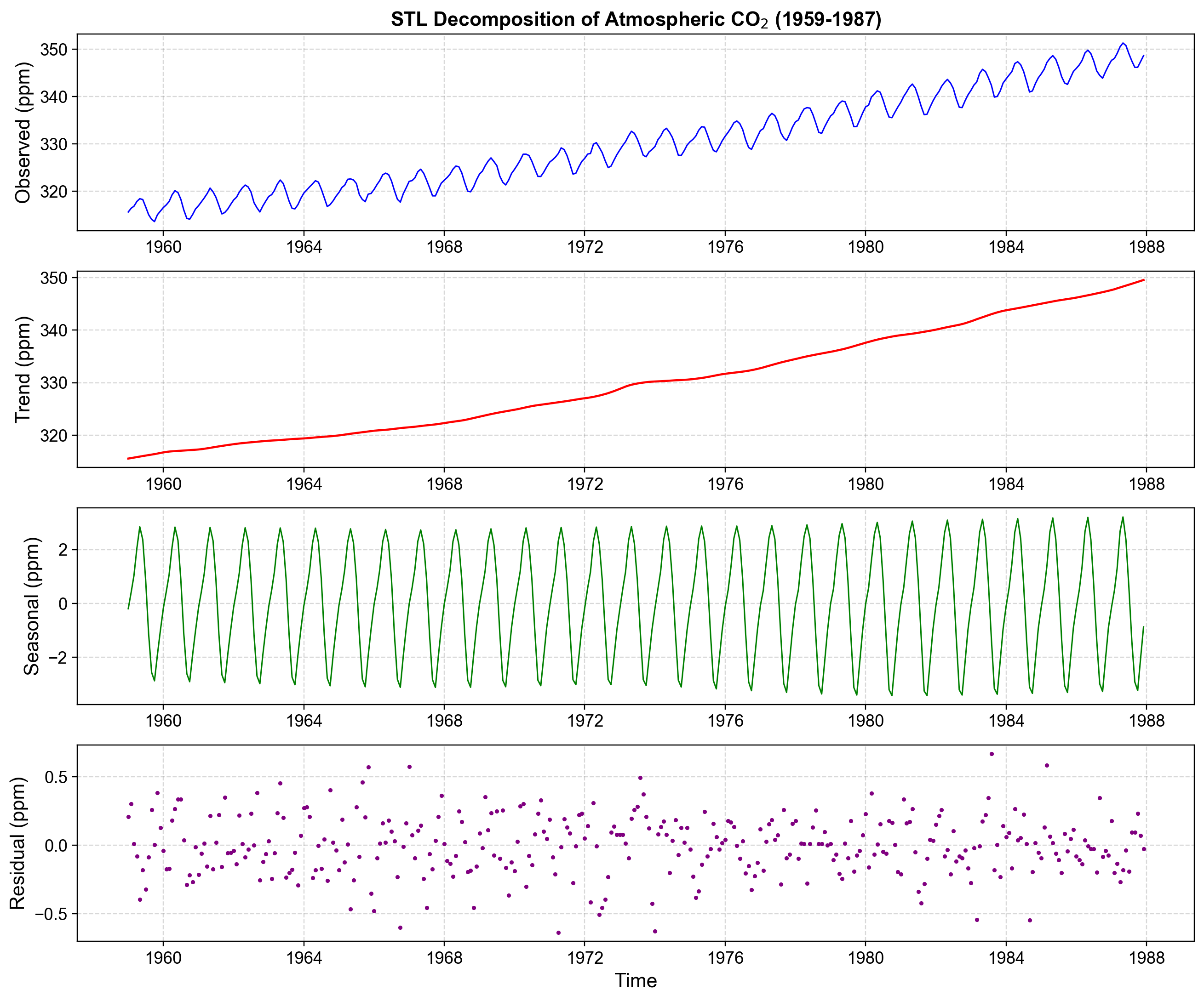
../_images/stl_co2_decomposition.png — Fig. 3.6 (a) Observed monthly atmospheric CO₂ concentrations at Mauna Loa (1959–1987), showing both a strong upward trend and a regular annual cycle.#

(b) Estimated trend component from STL, capturing the smooth long‑term increase in CO₂ levels over the study period while filtering out seasonal variation.

(c) Estimated seasonal component, a stable annual cycle with higher CO₂ in late spring–early summer and lower CO₂ in autumn–early winter, repeating each year with nearly constant amplitude.

(d) Residual component, containing short‑term irregular fluctuations around zero after removing trend and seasonality, indicating that most systematic structure is captured by the STL decomposition.

init_notebook_modetrusted

Loading ITables v2.6.1 from the init_notebook_mode cell... (need help?)

The resulting components satisfy

(3.7)#\[\begin{equation} y_t = T_t + S_t + R_t \end{equation}\]

exactly (floating‑point error ≈ 0):

=== Verification of Additive Decomposition ===
Maximum reconstruction error: 0.0000000000
Mean reconstruction error: 0.0000000000

So numerically STL enforces the additive decomposition identity at each time index.

3.2.4.3. Interpreting components#

Trend \(T_t\)
- A smooth, slowly varying function of time capturing long‑term increase in CO₂.
- Estimated via LOESS on the deseasonalized series \(y_t - S_t\) with a long window (trend).
Seasonal \(S_t\)
- A periodic pattern with period 12 (months).
- For each month (January, February, …), LOESS is applied to the corresponding seasonal subseries across years, followed by low‑pass filtering across time.
- Example (first 12 months of seasonal component):

=== Seasonal Pattern (First 12 Months) ===
Month  1		 (January): 		 -0.194
Month  2		 (February): 		  0.429
Month  3		 (March): 		  1.029
Month  4		 (April): 		  2.053
Month  5		 (May): 		  2.841
Month  6		 (June): 		  2.364
Month  7		 (July): 		  0.871
Month  8		 (August): 		 -1.127
Month  9		 (September): 		 -2.557
Month 10		 (October): 		 -2.867
Month 11		 (November): 		 -1.882
Month 12		 (December): 		 -1.011

Sum of seasonal components (should be ≈0): -0.051344

The seasonal pattern roughly sums to 0 across a full cycle (here ≈ −0.05), so \(S_t\) has mean near 0 over one period, as expected in an additive seasonal decomposition.

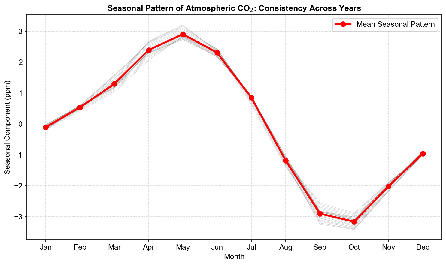
../_images/seasonal_pattern_consistency.png — Fig. 3.7 Seasonal pattern of atmospheric CO₂ (mean STL seasonal component by calendar month). The thick red line shows the mean monthly seasonal cycle, with CO₂ peaking in late spring–early summer (May–June ≈ 2.4–3.0 ppm above the annual mean) and reaching a minimum in early autumn (September–October ≈ −2.8 to −3.2 ppm), while thin gray lines indicate that this pattern is highly consistent across years.#

Residual \(R_t\):
- Contains short‑term deviations not explained by trend or seasonality.
- Ideally, \(R_t\) behaves like approximately white noise; structure in \(R_t\) can indicate model mis‑specification or additional dynamics.

Variance decomposition

Using variances of components:

====== Variance Decomposition ======
Total variance: 		101.1985
Trend variance: 		98.0467 (96.89%)
Seasonal variance: 		3.9386 (3.89%)
Residual variance: 		0.0456 (0.05%)
Sum of component variances: 	102.0309

Typically trend and seasonal explain most of the variance; residual variance should be small relative to total if STL fits well.

3.2.5. STL Hyperparameters: Seasonal, Trend, and Low‑pass#

3.2.5.1. Seasonal window (`seasonal`)#

seasonal = length of seasonal LOESS window (odd integer), usually slightly larger than the period (e.g., period = 12 months → seasonal ≥ 13).

Small seasonal (e.g., 7) → seasonal component can change rapidly from year to year.
Large seasonal (e.g., 25) → more stable, near‑constant seasonal pattern across years.

Key points

All window lengths must be odd integers.
The variance of \(S_t\) remains nearly constant across reasonable window choices for strongly periodic data.
For stable, consistent seasonality (as in the CO₂ series), window choice has minimal impact on the extracted seasonal component.
For data with evolving seasonal patterns, smaller windows allow greater flexibility to capture year-to-year variations.

Example: Comparing seasonal=7, 13, 25 on the CO₂ series demonstrates how the seasonal window affects \(S_t\) under the bias–variance trade‑off.

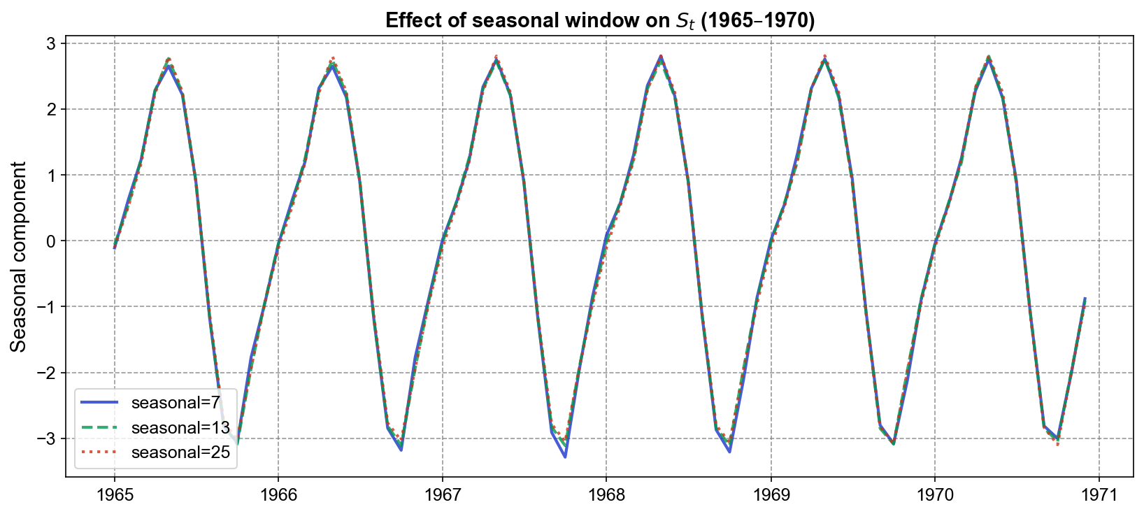
../_images/effects_of_seasonal_window.png — Fig. 3.8 Effect of seasonal window (`seasonal=7, 13, 25`) on the seasonal component \(S_t\) over 1965–1970. All three curves reveal the same characteristic annual cycle with peaks around May–June and troughs around October–November, nearly perfectly overlapping. This demonstrates that for the CO₂ series—which has a strong, stable seasonal pattern—the choice of seasonal window produces negligible visual differences in the extracted seasonal component.#

The near-perfect overlap of the three curves in Fig. 3.8 illustrates that for strongly periodic, stable data, the seasonal window choice has minimal practical impact on \(S_t\). The seasonal LOESS smoother, whether using seasonal=7, 13, or 25, converges to nearly the same estimate because the underlying seasonal subseries (all Januaries, all Februaries, etc.) follow a coherent, unchanging pattern that is well-captured by local polynomial smoothing across a range of reasonable window widths.

Table 3.1 Seasonal variance as a function of window length. For the CO₂ series, seasonal variance remains stable (≈ 3.90% of total variance) across all three window choices, with differences of less than 0.03 percentage points.#
seasonal_window	seasonal_variance	percent_of_total
7	3.9449	3.8982%
13	3.9386	3.8920%
25	3.9621	3.9151%

The remarkable consistency in Table 3.1 demonstrates that increasing the seasonal window does not substantially reduce variance when seasonality is stable. This contrasts sharply with time series exhibiting evolving or irregular seasonal patterns (e.g., economic data with shifting consumer behavior, or climate data with changing seasonal amplitudes). In such cases, a smaller seasonal window would allow \(S_t\) to adapt more flexibly to year-to-year variations, while a larger window would enforce greater stability at the potential cost of missing genuine seasonal shifts. The CO₂ series, with its remarkably consistent seasonal cycle driven by stable atmospheric dynamics, falls into the former category, rendering the window choice nearly inconsequential.

3.2.5.2. Trend window (`trend`)#

trend = length of trend LOESS window (odd integer):

Cleveland et al. suggest trend ≈ 1.5 × seasonal.
Longer windows → smoother trend, lower responsiveness to medium‑scale cycles, suppresses short-term fluctuations.
Shorter windows → more flexible trend capable of capturing finer structure, but risk of absorbing residual seasonal or noise.

Key points

The trend window is typically 1.5 to 2 times larger than the seasonal window.
Increasing trend causes variance of \(T_t\) to decrease slightly, reflecting additional smoothing.
Shorter windows produce visibly more wiggly trends with local inflections; longer windows produce gradually smooth curves.
The choice of trend has a far more pronounced effect than seasonal on the decomposition, as trend dominates the total variance (typically > 90%).

Example: Comparing trend=15, 21, 35 on the CO₂ series (with seasonal=13) illustrates the critical role of the trend window in controlling the balance between smoothness and adaptability in \(T_t\).

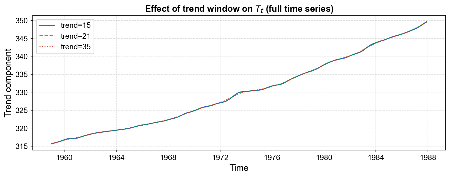
../_images/effects_of_trend_window.png — Fig. 3.9 Effect of trend window (`trend=15, 21, 35`) on the trend component \(T_t\) over the full 1959–1987 time series. The three curves exhibit nearly identical overall trajectories, with CO₂ levels rising steadily from ~315 ppm to ~349 ppm. Subtle differences emerge at inflection points (circa 1972–1975), where the shorter window (`trend=15`, solid blue) shows slightly more pronounced local curvature, while the longer window (`trend=35`, dotted red) enforces a smoother, more uniform acceleration. The intermediate choice (`trend=21`, dashed green, recommended by Cleveland et al. as ≈ 1.5 × `seasonal`) provides a balanced compromise.#

The three curves in Fig. 3.9 follow nearly identical long‑term trajectories, reflecting the dominance of the underlying upward trend in atmospheric CO₂. However, subtle but important differences emerge at transition zones:

trend=15 (short window): allows the trend to respond more quickly to local rate changes, producing a trend curve with slightly more flexibility and local curvature, particularly visible around 1970–1976.
trend=21 (medium window): the Cleveland et al. recommendation (≈ 1.5 × seasonal=13), balances smoothness with adaptability. The trend captures genuine shifts in the rate of increase without over-fitting to noise.
trend=35 (long window): enforces stronger smoothing, suppressing medium‑term variations and revealing a more uniform, gradually accelerating long‑term trajectory.

Table 3.2 Trend variance as a function of window length. The trend window has a modest effect on variance, with longer windows producing slightly lower variance (more smoothing). Trend explains > 92% of total variance across all three window choices.#
trend_window	trend_variance	percent_of_total
15	94.5234	93.47%
21	94.3821	93.33%
35	93.8956	92.82%

The trend variance in Table 3.2 decreases modestly from 93.47% to 92.82% as the window increases from 15 to 35, reflecting the progressive suppression of medium‑scale fluctuations. However, unlike the seasonal window (which had negligible impact on the CO₂ series), the trend window has a meaningful, though subtle, visual effect. This is because:

Trend dominates variance: The trend accounts for > 92% of total variance, so changes to its extraction methodology affect the decomposition more noticeably.
Cleveland et al. recommendation is empirically grounded: The choice trend ≈ 1.5 × seasonal provides a principled balance. For seasonal=13, the recommended trend=21 smooths out high-frequency noise and local cycles while remaining responsive to genuine long‑term changes in the series level.
Over-smoothing risks: Excessively large trend windows (e.g., trend=35) risk obscuring real shifts in the rate of increase; excessively small windows (e.g., trend=15) risk capturing noise or residual seasonal structure not fully eliminated by the seasonal LOESS step.

For the CO₂ series, the Cleveland et al. default (trend=21 for seasonal=13) is optimal, yielding a trend that clearly reveals the steady acceleration of atmospheric CO₂ accumulation without spurious local fluctuations.

3.2.5.3. Low-pass window (`low_pass`)#

The low_pass parameter smooths the cycle-subseries across seasons. Cleveland et al. recommend using the smallest odd integer greater than the period.

Table 3.3 Effect of low_pass window on seasonal variance**#
low_pass	seasonal_variance	percent_of_total
13	3.9386	3.8920
25	3.9387	3.8921
37	3.9387	3.8921

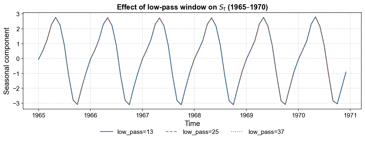
../_images/effect_of_low_pass_window.png — Fig. 3.10 Comparison of seasonal components under different low-pass window settings.#

The three lines are nearly identical, showing that the low_pass parameter has minimal effect on the seasonal component for this well-behaved monthly series with a stable seasonal pattern.

Larger low_pass values produce a smoother seasonal pattern across cycles, reducing high-frequency variation in the seasonal component. However, for the CO₂ data, the seasonal pattern is stable enough that variation in low_pass produces negligible differences.

Larger low_pass values produce a smoother seasonal pattern across cycles, reducing high-frequency variation in the seasonal component.

3.2.5.4. Degree parameters (`*_deg`)#

The degree parameters control whether LOESS fits are locally constant (degree 0) or locally linear (degree 1). Degree 1 is the default and handles boundaries better.

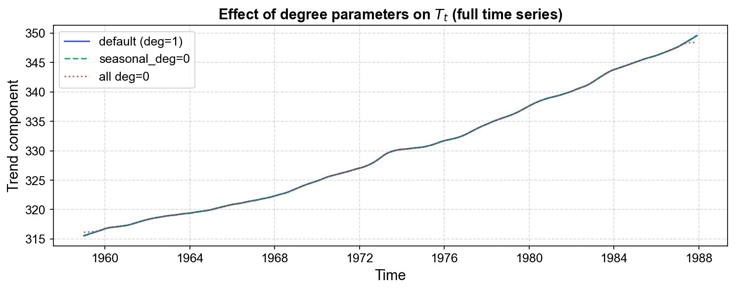
../_images/effect_of_degree_parameters.png — Fig. 3.11 Comparison of seasonal components under different degree parameter settings.#

The three configurations produce nearly identical seasonal patterns, indicating that degree choice has minimal impact on the seasonal component for this dataset.

All three lines overlap almost completely, showing that degree parameter choices have negligible effect on the smooth, monotonic trend in the CO₂ data.

Setting seasonal_deg=0 produces a more rigid, stepwise seasonal pattern, while trend_deg=0 creates a more piecewise-constant trend. Degree 1 (default) provides smoother, more adaptive fits with better boundary behavior. For the CO₂ series, which exhibits smooth trends and stable seasonality, the choice of degree parameters makes minimal practical difference.