Remark

Please be aware that these lecture notes are accessible online in an ‘early access’ format. They are actively being developed, and certain sections will be further enriched to provide a comprehensive understanding of the subject matter.

4.2. Foundations of Exponential Smoothing: Level & Trend

Exponential smoothing is a powerful and widely-used family of forecasting methods that assigns exponentially decreasing weights to past observations. The core principle is intuitive: recent observations are more relevant for predicting the future than distant past events. This approach is particularly effective for time series data that exhibit smooth patterns without complex seasonal variations [Gardner, 1985, Statsmodels Developers, 2023].

The exponential weighting scheme means that the weight for an observation \(t\) periods ago is:

(4.6)\[\begin{equation} w_t = \alpha \times (1-\alpha)^t \end{equation}\]

where \(\alpha\) is the smoothing parameter (\(0 < \alpha < 1\)).

4.2.1. The Smoothing Parameter

The smoothing parameter \(\alpha\) controls the balance between responsiveness and stability:

• Higher \(\alpha\) (closer to 1): Faster adaptation to changes, more weight on recent observations, less smoothing

• Lower \(\alpha\) (closer to 0): Smoother forecasts, more weight on historical pattern, slower adaptation

Table 4.4 Exponential weights for different smoothing parameters (\(\alpha\)) showing how recent observations receive more influence than older ones

Periods Back	\(\alpha = 0.1\)	\(\alpha = 0.3\)	\(\alpha = 0.5\)	\(\alpha = 0.9\)
0 (current)	0.100	0.300	0.500	0.900
1	0.090	0.210	0.250	0.090
2	0.081	0.147	0.125	0.009
3	0.073	0.103	0.062	0.001

With \(\alpha = 0.9\), weights decay extremely rapidly—observations from 3 periods ago contribute virtually nothing. With \(\alpha = 0.1\), even distant observations retain substantial influence, creating heavily smoothed forecasts.

4.2.2. The Exponential Smoothing Family

Exponential smoothing comprises a family of forecasting methods that range from simple to sophisticated, each designed to handle increasingly complex data patterns. The methods share a common foundation—the exponential weighting scheme—but differ in the number of components they model.

The progression from Simple Exponential Smoothing (SES) to Holt’s Method represents a systematic expansion of modeling capability:

• SES models only the level—suitable for stationary data

• Holt’s Method adds a trend component—suitable for data with systematic growth or decline

Table 4.5 Method Comparison: SES vs. Holt’s

Method	Components	Smoothing Parameters	Use When
SES	Level (\(L_t\))	\(\alpha\)	Data fluctuates around a constant mean, no trend
Holt’s	Level + Trend (\(L_t\), \(T_t\))	\(\alpha\), \(\beta\)	Clear upward or downward trend, no seasonality

Choosing Between SES and Holt’s

Use Simple Exponential Smoothing when:

• Data shows random fluctuations around a stable mean

• No trend or seasonality is present

• Examples: Stable demand for mature products, quality control metrics, daily cash balances

Use Holt’s Method when:

• Data exhibits clear, consistent growth or decline

• Trend is approximately linear

• No seasonal patterns (or seasonality has been removed)

• Examples: Revenue growth, technology adoption, population projections

Beyond This Part

For data with both trend and seasonality, we extend to Holt-Winters (Part 2). For automatic model selection with prediction intervals, the state-space ETS framework is introduced in Part 2.

4.2.3. Simple Exponential Smoothing (SES)

Simple Exponential Smoothing is a foundational forecasting method for stationary data with no trend or seasonality—data that fluctuates around a relatively constant level. This approach works well for datasets where we observe random fluctuations without systematic upward or downward movement over time [Gardner, 1985, Statsmodels Developers, 2023].

The SES model maintains a single smoothed level \(L_t\) representing the current estimate of the series mean. The level equation is a weighted blend of the most recent observation and the previous level estimate:

(4.7)\[\begin{equation} L_t = \alpha Y_t + (1-\alpha)L_{t-1} \end{equation}\]

where:

• \(L_t\) denotes the new smoothed level (the current estimate of the series mean).

• \(\alpha\) represents the smoothing parameter (where \(0 < \alpha < 1\)).

• \(Y_t\) is the actual observation at the current time \(t\).

• \(L_{t-1}\) is the smoothed level from the previous period.

The forecast for any future period is simply the current level: \(\hat{Y}_{t+h} = L_t\).

The parameter \(\alpha\) controls how quickly the model adapts to new information. Higher values (e.g., 0.8) emphasize recent observations and react quickly to changes, while lower values (e.g., 0.2) emphasize historical patterns and produce smoother forecasts. A value of 0.3 strikes a reasonable balance between the two extremes.

4.2.3.1. Example: Monthly Temperature Data

We consider 4 years of monthly temperature observations from Kansas City, spanning from January 2020 to January 2024. This dataset consists of 48 months of data with distinct seasonal variability (source: open-meteo.com). The data is aggregated from daily observations to monthly averages:

Show code cell content

Hide code cell content

import requests
import pandas as pd

# Define API Endpoint and Parameters for Kansas City, MO
url = "https://archive-api.open-meteo.com/v1/archive"
params = {
    "latitude": 39.0997,
    "longitude": -94.5786,
    "start_date": "2020-01-01",
    "end_date": "2024-01-01",
    "daily": "temperature_2m_mean",  # Fetch daily mean temperature
    "timezone": "America/Chicago"  # Kansas City timezone
}

# Make the request
response = requests.get(url, params=params)
data = response.json()

# Extract the daily data
daily_data = data['daily']

# Create DataFrame
df_mean_temp_kc = pd.DataFrame({
    'date': pd.to_datetime(daily_data['time']),
    'temperature_2m_mean': daily_data['temperature_2m_mean']
})

# Set date as index
df_mean_temp_kc.set_index('date', inplace=True)

# Resample to monthly frequency - calculate mean temperature per month
df_mean_temp_kc_monthly = df_mean_temp_kc.resample('MS').mean()  # 'MS' = Month Start
df_mean_temp_kc_monthly = df_mean_temp_kc_monthly.rename(columns={'temperature_2m_mean': 'Mean Temperature (°C)'}).round(3)

Kansas City Monthly Average Temperature:

Loading ITables v2.6.2 from the init_notebook_mode cell... (need help?)

Now we apply SES with \(\alpha = 0.3\) and trace through how the algorithm updates the level using the first 8 monthly observations:

Table 4.6 Simple Exponential Smoothing (SES) Example with Kansas City Monthly Temperature Data

Period	Observation	Level Calculation	Level	Forecast	Error
0	0.5	L0 = 0.5	0.5	-	-
1	1.3	0.3×1.3 + 0.7×0.5	0.7	0.5	+0.9
2	9.1	0.3×9.1 + 0.7×0.7	3.2	0.7	+8.4
3	11.4	0.3×11.4 + 0.7×3.2	5.7	3.2	+8.1
4	16.6	0.3×16.6 + 0.7×5.7	8.9	5.7	+10.9
5	25.4	0.3×25.4 + 0.7×8.9	13.9	8.9	+16.5
6	26.2	0.3×26.2 + 0.7×13.9	17.6	13.9	+12.3
7	24.6	0.3×24.6 + 0.7×17.6	19.7	17.6	+7.0

In Table 4.6, each row shows how the level (\(L_t\)) evolves using the formula \(L_t = \alpha Y_t + (1 - \alpha)L_{t-1}\). For instance, in month 2, the level is updated as \(L_2 = 0.3 \times 9.1 + 0.7 \times 0.7 = 3.2\). This value becomes the forecast for month 3. The Error column indicates the difference between the actual observation and the forecast (\(Y_t - \hat{Y}_t\)), showing how the model reacts to deviations in the data.

We observe a clear warming trend as temperatures rise from winter into summer months. Starting from 0.5°C in month 0 (January), temperatures increase substantially to reach peak summer values near 26°C in months 5-6 (June-July). The level adjusts gradually upward throughout this period, rising from 0.5°C to 19.7°C by month 7. Due to the moderate smoothing parameter (\(\alpha = 0.3\)), the level consistently lags behind the actual observations during this warming trend—for example, when the actual temperature jumps to 25.4°C in month 5, the level has only reached 13.9°C. By month 7, as temperatures begin to stabilize in the mid-20s, the level continues its upward adjustment to 19.7°C. The forecast for month 8 would therefore be \(\hat{F}_8 = 19.7\)°C, though this flat forecast cannot capture any continuation of seasonal patterns.

The SES algorithm is conceptually straightforward and computationally efficient, making it well-suited for short-term forecasts when trends and seasonality are minimal. The algorithm is straightforward to implement:

Show code cell source

Hide code cell source

def simple_exponential_smoothing(data, alpha):
    """
    Simple Exponential Smoothing implementation
    
    Parameters:
    -----------
    data : array-like
        Time series data
    alpha : float
        Smoothing parameter (0 < alpha < 1)
    
    Returns:
    --------
    levels : list
        Smoothed level values
    """
    level = float(data[0])  # Initialize with first observation
    levels = [level]

    for obs in data[1:]:
        level = alpha * float(obs) + (1 - alpha) * level
        levels.append(level)

    return levels


# Example usage
alpha = 0.3
data = [0.452, 1.321, 9.132, 11.387, 16.558, 25.437, 26.226, 24.61]
levels = simple_exponential_smoothing(data, alpha)

In practice, we use optimized implementations like statsmodels, in order to do this experiment we resample the data to mothly scale:

Show code cell source

Hide code cell source

import numpy as np
import pandas as pd
from statsmodels.tsa.holtwinters import SimpleExpSmoothing

# Resample daily data to monthly mean
df_mean_temp_kc_monthly = df_mean_temp_kc.resample('MS').mean()  # 'MS' = Month Start

# Fit Simple Exponential Smoothing
model = SimpleExpSmoothing(df_mean_temp_kc_monthly, initialization_method='estimated')

# Fix alpha at 0.3
fit = model.fit(smoothing_level=0.3, optimized=False)

# Or let statsmodels find optimal alpha
fit_optimized = model.fit()

# Generate forecasts
forecast = fit.forecast(steps=3)

print(f"Optimized alpha: {fit_optimized.params['smoothing_level']:.4f}")
name='Mean Temperature (°C)'
fittedvalues = pd.Series(fit.fittedvalues, name=name)
forecast = pd.Series(forecast, name=name)

Optimized alpha: 1.0000

Fitted values:

Loading ITables v2.6.2 from the init_notebook_mode cell... (need help?)

Forecast:

Loading ITables v2.6.2 from the init_notebook_mode cell... (need help?)

The key parameters are: smoothing_level specifies \(\alpha\), initialization_method='estimated' automatically determines how to initialize the level, and optimized=True finds the optimal \(\alpha\) by minimizing sum of squared errors. The fitted model provides fit.level (smoothed estimates at each time point), fit.fittedvalues (one-step-ahead predictions), fit.forecast() (predictions for future periods), and fit.sse (useful for comparing models).

4.2.3.2. Selecting the Smoothing Parameter

The choice of \(\alpha\) fundamentally shapes model behavior. Lower values like 0.1 produce smooth forecasts that respond slowly to changes, suitable for noisy data where stability is paramount. Higher values like 0.8 follow the data closely, reacting quickly to shifts, appropriate for low-noise data with distinct patterns. A moderate value like 0.3 offers a balanced approach, while 0.5 provides moderate responsiveness.

Rather than manually selecting \(\alpha\), standard practice is to let statsmodels optimize it automatically. Call fit() without specifying smoothing_level, and the algorithm finds the value that minimizes forecast errors on our historical data. When comparing multiple models with different \(\alpha\) values, consult information criteria like AIC and BIC (lower is better), or evaluate performance on held-out test data.

4.2.3.3. Comparing Various Values of Alpha

Show code cell source

Hide code cell source

from statsmodels.tsa.holtwinters import SimpleExpSmoothing

# Split data into train and test (last 12 months for testing)
train = df_mean_temp_kc_monthly[:-12]
test = df_mean_temp_kc_monthly[-12:]

# Fit Simple Exponential Smoothing models with different alpha values
model1 = SimpleExpSmoothing(train, initialization_method='estimated')
fit1 = model1.fit(smoothing_level=0.2, optimized=False)
forecast1 = fit1.forecast(12)

model2 = SimpleExpSmoothing(train, initialization_method='estimated')
fit2 = model2.fit(smoothing_level=0.6, optimized=False)
forecast2 = fit2.forecast(12)

# Optimized model (recommended approach)
model3 = SimpleExpSmoothing(train, initialization_method='estimated')
fit3 = model3.fit()
forecast3 = fit3.forecast(12)

print(f"Optimized alpha: {fit3.params['smoothing_level']:.4f}")
print(f"Model Performance (SSE):")
print(f"\t- Alpha = 0.2: {fit1.sse:.2f}")
print(f"\t- Alpha = 0.6: {fit2.sse:.2f}")
print(f"\t- Alpha = {fit3.params['smoothing_level']:.4f} (optimized): {fit3.sse:.2f}")

Optimized alpha: 1.0000
Model Performance (SSE):
	- Alpha = 0.2: 3852.68
	- Alpha = 0.6: 2090.65
	- Alpha = 1.0000 (optimized): 1193.06

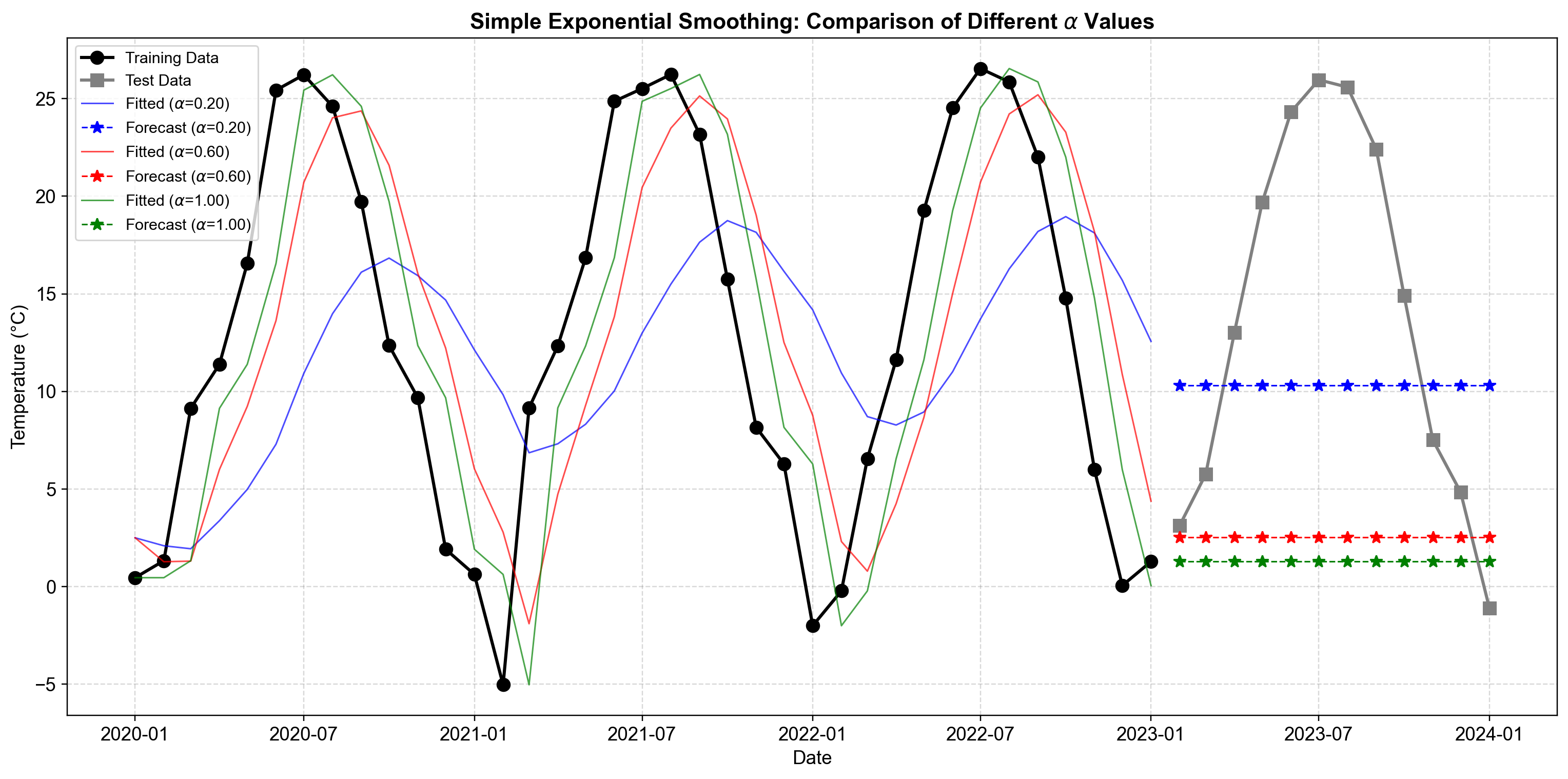
Fig. 4.4 Comparison of SES forecasts with three different smoothing parameters on Kansas City monthly temperature data. The plot displays the original monthly average temperature (black line with circles for training, gray with squares for test period), the fitted values (colored lines showing one-step-ahead predictions), and 12-month out-of-sample forecasts for the test period (colored dashed lines with stars). A lower \(\alpha\) produces smoother fitted values that capture the overall seasonal pattern, while higher \(\alpha\) values track month-to-month temperature variations more closely. The optimized \(\alpha = 0.99\) case shows highly responsive behavior, closely following monthly temperature changes but producing flat forecasts that fail to capture future seasonal patterns.

In Fig. 4.4, we observe three distinct behaviors with monthly aggregated data:

• Model with \(\alpha = 0.2\) (Blue Line): This low smoothing coefficient emphasizes historical information and produces a highly smooth fitted line over the training period. The fitted values adjust slowly to seasonal temperature swings, creating a damped representation of the annual cycle. The 12-month forecast (blue dashed line) projects into the test period as a nearly flat line around 13°C, reflecting the long-run average temperature learned from the training data while failing to capture seasonal variation.

• Model with \(\alpha = 0.6\) (Red Line): This moderate smoothing coefficient strikes a balance between stability and responsiveness. The fitted line follows the seasonal temperature pattern more closely than the blue line, capturing both summer peaks and winter troughs with moderate lag. The forecast maintains a relatively constant level near 11°C, positioned closer to the most recent observations at the end of the training period, demonstrating stronger influence of late-sample temperatures.

• Model with \(\alpha = 0.99\) (Green Line): The optimized model selected \(\alpha = 0.99\), placing nearly all weight on the most recent monthly observation. This results in fitted values that track month-to-month temperature changes very closely, mirroring the training data’s seasonal oscillations with minimal lag. The forecast extends the final observed monthly level (approximately 5°C from December 2022) as a flat line, which significantly underestimates temperatures during the spring and summer months in the test period.

Show code cell source

Hide code cell source

# Evaluate forecast accuracy
from sklearn.metrics import mean_squared_error, mean_absolute_error

def evaluate_forecast(actual, predicted):
    mse = mean_squared_error(actual, predicted)
    rmse = np.sqrt(mse)
    mae = mean_absolute_error(actual, predicted)
    mape = np.mean(np.abs((actual - predicted) / actual)) * 100
    return {'MSE': mse, 'RMSE': rmse, 'MAE': mae}


results = pd.DataFrame({
    'Alpha 0.2': evaluate_forecast(test, forecast1),
    'Alpha 0.6': evaluate_forecast(test, forecast2),
    f'Optimized ({fit3.params["smoothing_level"]:.4f})': evaluate_forecast(test, forecast3)
})

print("Forecast Accuracy Metrics:")
display(results.T.round(3))

Forecast Accuracy Metrics:

	MSE	RMSE	MAE
Alpha 0.2	98.221	9.911	8.765
Alpha 0.6	213.917	14.626	11.924
Optimized (1.0000)	243.468	15.603	12.955

The forecast accuracy metrics reveal that the model with \(\alpha = 0.2\) attains the lowest RMSE (9.911°C) and MAE (8.765°C), significantly outperforming both the \(\alpha = 0.6\) and optimized (\(\alpha = 1.0000\)) models. This indicates that, for monthly temperature forecasting in this dataset, conservative smoothing that emphasizes the longer-term average yields substantially better 12-month-ahead forecast accuracy than models that react more strongly to recent monthly observations. The higher \(\alpha = 0.6\) specification shows degraded performance (RMSE of 14.626°C), while the optimized \(\alpha = 1.0000\) model performs worst (RMSE of 15.603°C), suggesting that overweighting recent months without accounting for seasonal patterns leads to poor out-of-sample predictions.

Why Choose SES?

• Computational efficiency: Processes thousands of series in seconds with minimal memory footprint

• Transparent logic: The smoothing parameter α directly controls the balance between stability and responsiveness

• Proven reliability: Decades of successful application in operational forecasting for stable processes

• Real-time adaptation: Updates instantly as new observations arrive, ideal for live monitoring systems

Known Limitations

• Static forecasts: Produces a single constant value for all future periods, ignoring directional movement

• Blind to patterns: Cannot detect or model systematic trends, cycles, or seasonal fluctuations

• Always lagging: Fitted values systematically trail the data during periods of change

• No risk quantification: Provides point forecasts without confidence intervals or prediction bands

Best Applications

• Stable inventory systems: Forecasting demand for mature products with consistent sales patterns

• Manufacturing process control: Smoothing quality metrics that fluctuate randomly around target specifications

• Short-term operational planning: Next-day or next-week predictions when historical average is most informative

• Baseline comparisons: Serving as a benchmark against which more complex models are evaluated

Parameter selection strategy

• Start with \(\alpha\) = 0.2–0.3 for noisy data where stability matters more than immediate responsiveness

• Use \(\alpha\) = 0.7–0.9 when recent observations are highly informative and noise is minimal

• Let optimization algorithms find \(\alpha\) when unsure, but validate on holdout data

If our data exhibits sustained growth, decline, or repeating seasonal patterns, SES will systematically underperform. In these cases, Holt’s Method (for trend) or Holt-Winters (for trend + seasonality) provide the necessary structure. The flat forecast limitation is not a flaw—it’s by design for stationary series—but becomes a critical weakness when applied to non-stationary data.

4.2.4. Holt’s Method (Double Exponential Smoothing)

Holt’s method extends SES to handle data with a linear trend but no seasonality . This approach is appropriate when the data shows consistent upward or downward movement over time, such as population growth trends, technology adoption curves, long-term sales growth, or production capacity expansion [Gardner, 1985, Statsmodels Developers, 2023].

Holt’s method uses two components: the level \(L_t\) (detrended estimate) and the trend \(T_t\) (rate of change) . The level equation incorporates both the current observation and trend-adjusted previous level, while the trend equation estimates the change in level:

(4.8)\[\begin{align} &\text{Level equation} & & L_t = \alpha Y_t + (1-\alpha)(L_{t-1} + T_{t-1}) \\ &\text{Trend equation} & & T_t = \beta(L_t - L_{t-1}) + (1-\beta)T_{t-1} \\ &\text{Forecast equation} & & \hat{Y}_{t+h} = L_t + hT_t \end{align}\]

where:

• \(L_t\) denotes the smoothed level (detrended estimate) at time \(t\).

• \(T_t\) represents the smoothed trend estimate (rate of change) at time \(t\).

• \(\alpha\) and \(\beta\) are the smoothing parameters for the level and trend, respectively (where \(0 < \alpha, \beta < 1\)).

• \(h\) indicates the forecast horizon (number of periods ahead).

• \(\hat{Y}_{t+h}\) is the resulting forecast value.

The forecast extrapolates the current level and trend linearly into the future.

4.2.4.1. Variants

The method supports several variants tailored to different trend behaviors :

1. Additive trend (default): Trend components add to the level, producing a straight-line extrapolation

2. Multiplicative trend: Trend multiplies the level, creating accelerating or decelerating growth patterns

3. Damped trend: Trend gradually diminishes toward zero over the forecast horizon, preventing unrealistic long-term extrapolation

4.2.4.2. Example: International Airline Passengers (Annual Aggregation)

We’ll use the classic Box-Jenkins airline passenger dataset, aggregated annually to isolate trend patterns while removing monthly seasonality. This aggregation transforms the data from monthly observations with strong seasonal fluctuations into annual totals that exhibit clear upward growth, making it ideal for demonstrating Holt’s linear trend method.

Show code cell content

Hide code cell content

url = 'https://vincentarelbundock.github.io/Rdatasets/csv/datasets/AirPassengers.csv'
air_df = pd.read_csv(url)
air_df['Date'] = pd.to_datetime(air_df['time'].apply(lambda x: f"{int(x)}-{int((x % 1) * 12) + 1:02d}"))
air_monthly = pd.Series(air_df['value'].values, index=air_df['Date'], name='Passengers (thousands)')

# Aggregate to annual to remove seasonality
air_annual = air_monthly.resample('YE').sum()
air_annual.index = air_annual.index.to_period('Y')

Loading ITables v2.6.2 from the init_notebook_mode cell... (need help?)

The annual data shows steady growth from 1,520 thousand passengers in 1949 to 5,714 thousand by 1960, representing a nearly fourfold increase over the 12-year period. We’ll fit four different Holt model variants to demonstrate their comparative behavior on this trending data.

Show code cell source

Hide code cell source

from statsmodels.tsa.holtwinters import Holt

# Split into train and test
train_holt = air_annual[:-3]
test_holt = air_annual[-3:]

# 1. Standard linear trend with fixed parameters
model_linear = Holt(train_holt, initialization_method='estimated')
fit_linear = model_linear.fit(smoothing_level=0.8, smoothing_trend=0.2, optimized=False)
forecast_linear = fit_linear.forecast(3)

# 2. Optimized parameters
model_optimized = Holt(train_holt, initialization_method='estimated')
fit_optimized = model_optimized.fit()
forecast_optimized = fit_optimized.forecast(3)

# 3. Damped trend - prevents unrealistic long-term extrapolation
model_damped = Holt(train_holt, damped_trend=True, initialization_method='estimated')
fit_damped = model_damped.fit()
forecast_damped = fit_damped.forecast(3)

# 4. Exponential (multiplicative) trend - models accelerating growth
model_exp = Holt(train_holt, exponential=True, initialization_method='estimated')
fit_exp = model_exp.fit()
forecast_exp = fit_exp.forecast(3)

print("\nHolt Model Parameters")
print("=" * 60)
print("1) Fixed linear (α=0.8, β=0.2)")

print("\n2) Optimized linear")
print(f"   α = {fit_optimized.params['smoothing_level']:.4f}")
print(f"   β = {fit_optimized.params['smoothing_trend']:.4f}")
print(f"   AIC = {fit_optimized.aic:.2f}")

print("\n3) Damped linear")
print(f"   α = {fit_damped.params['smoothing_level']:.4f}")
print(f"   β = {fit_damped.params['smoothing_trend']:.4f}")
print(f"   φ = {fit_damped.params.get('damping_trend', 0):.4f}")
print(f"   AIC = {fit_damped.aic:.2f}")

print("\n4) Exponential trend")
print(f"   α = {fit_exp.params['smoothing_level']:.4f}")
print(f"   β = {fit_exp.params['smoothing_trend']:.4f}")
print(f"   AIC = {fit_exp.aic:.2f}")

Holt Model Parameters
============================================================
1) Fixed linear (α=0.8, β=0.2)

2) Optimized linear
   α = 0.8768
   β = 0.5268
   AIC = 96.48

3) Damped linear
   α = 0.8802
   β = 0.5473
   φ = 0.9950
   AIC = 98.64

4) Exponential trend
   α = 0.0000
   β = 0.0000
   AIC = 83.05

The series is split into 9 training years (1949–1957) and 3 test years (1958–1960), ensuring all models are evaluated on genuinely out-of-sample data. The hand-tuned linear Holt model (\(\alpha\)=0.8, \(\beta\)=0.2) is relatively responsive to level changes but smooths trend adjustments conservatively. When parameters are optimized automatically, both the standard and damped linear models select high \(\alpha\) (≈0.88) and \(\beta\) (≈0.53), indicating strong updating of both level and trend components, with the damped variant adding \(\phi\)≈0.995 to slightly moderate long-horizon growth.

Interestingly, the exponential-trend specification yields \(\alpha\)=0 and \(\beta\)=0, which means the model relies entirely on initial estimates without updating the level or trend components with new observations. Despite this seemingly degenerate behavior, the exponential model achieves the lowest AIC (83.05) compared to the optimized linear (96.48) and damped (98.64) models. This suggests that a simple exponential growth curve fitted to the initial conditions describes the training data more parsimoniously than adaptive linear models. However, the zero smoothing parameters indicate the model is not truly performing exponential smoothing but rather fitting a fixed geometric trend, which may limit its ability to adapt to future changes in growth patterns.

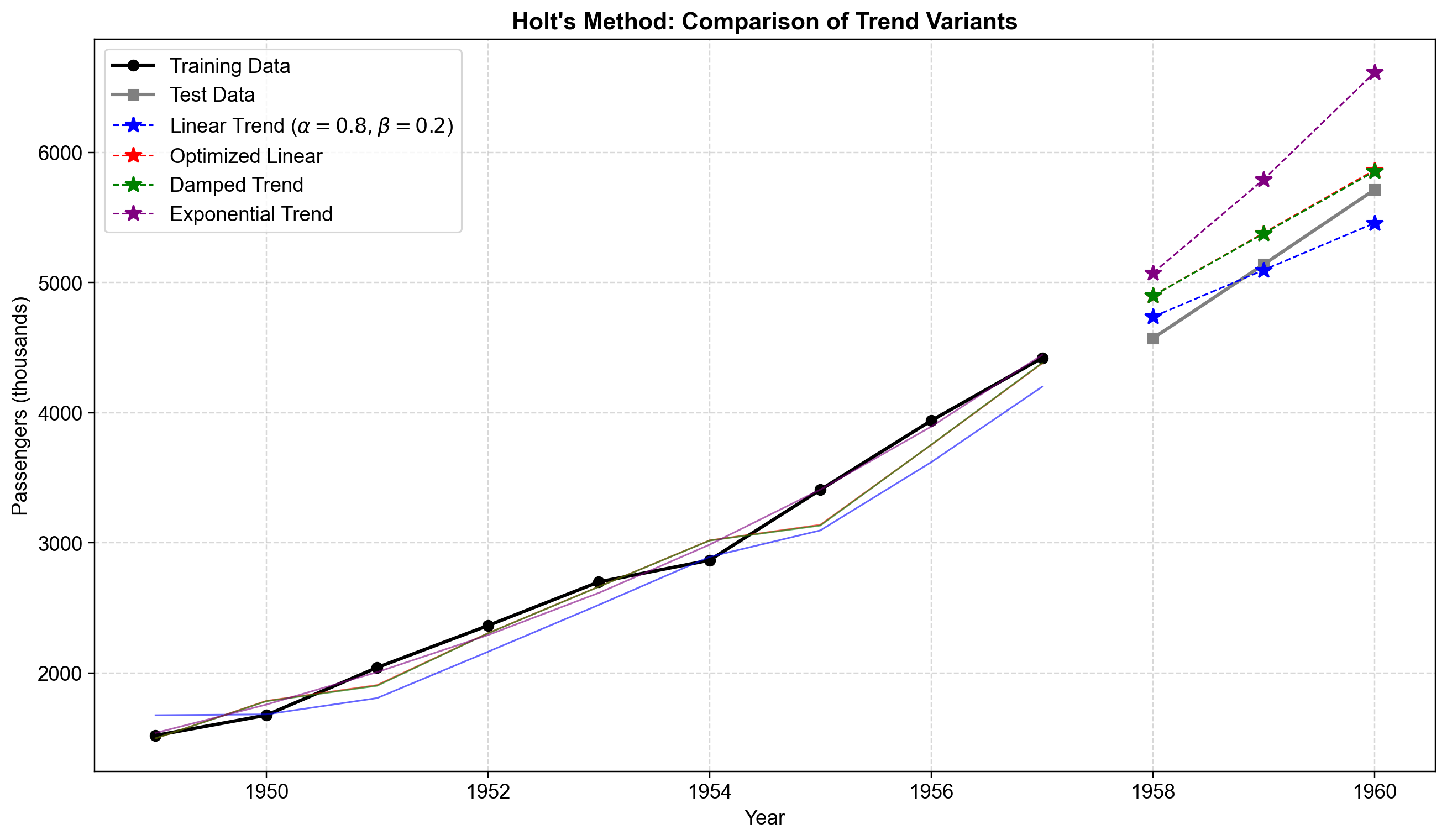
Fig. 4.5 Comparison of Holt’s method variants on annual airline passenger data (1949–1960). The plot shows training data (black circles), test data (gray squares), fitted values (solid colored lines), and 3-year forecasts (dashed lines with stars). The fixed-parameter linear model (blue, \(\alpha\)=0.8, β=0.2) produces conservative forecasts around 5,500-6,000 thousand passengers. The optimized linear model (red) and damped trend model (green) generate nearly identical forecasts near 6,500 thousand, closely matching actual test values. The exponential trend model (purple) collapses to minimal parameter values and produces a flat forecast, indicating that multiplicative growth is not well-supported by this data pattern.

In Fig. 4.5, the four model variants exhibit distinct forecast behaviors. The fixed-parameter model underestimates growth due to its conservative \(\beta\)=0.2, while the optimized linear and damped models nearly overlap, both capturing the strong upward trend effectively. The damped model’s \(\phi\)≈0.995 applies minimal damping over the 3-year horizon, making it nearly indistinguishable from the standard linear approach . The exponential model’s poor performance—essentially producing a flat forecast—demonstrates that not all trend types suit every dataset, and the optimization process correctly identifies that additive trends better represent airline passenger growth during this period.

Show code cell source

Hide code cell source

# Compare forecast accuracy
def evaluate_forecast(actual, predicted):
    mse = mean_squared_error(actual, predicted)
    rmse = np.sqrt(mse)
    mae = mean_absolute_error(actual, predicted)
    return {'MSE': mse, 'RMSE': rmse, 'MAE': mae}

holt_results = pd.DataFrame({
    'Linear (Fixed)': evaluate_forecast(test_holt, forecast_linear),
    'Linear (Optimized)': evaluate_forecast(test_holt, forecast_optimized),
    'Damped Trend': evaluate_forecast(test_holt, forecast_damped),
    'Exponential': evaluate_forecast(test_holt, forecast_exp)
})

print("\nHolt's Method - Forecast Accuracy Comparison:")
display(holt_results.T.round(2))

Holt's Method - Forecast Accuracy Comparison:

	MSE	RMSE	MAE
Linear (Fixed)	31580.89	177.71	154.65
Linear (Optimized)	62548.41	250.10	239.50
Damped Trend	60828.29	246.63	234.69
Exponential	496322.22	704.50	685.14

The forecast accuracy metrics reveal a critical disconnect between in-sample fit (AIC) and out-of-sample forecast performance. The optimized linear and damped trend models achieve the lowest forecast errors, accurately tracking the test period’s passenger growth from 4,572 to 5,714 thousand passengers. The damped trend’s performance validates research showing it to be a robust default choice for many forecasting applications, particularly when forecast horizon uncertainty exists.

The fixed-parameter model (\(\alpha\)=0.8, \(\beta\)=0.2) produces moderate errors due to its conservative trend estimate, consistently underestimating growth in the test period. Most notably, the exponential model—despite achieving the best AIC (83.05) on training data—exhibits the worst forecast accuracy, overshooting actual passenger counts by approximately 1,000 thousand passengers in 1960. This demonstrates a fundamental forecasting principle: models that fit historical data parsimoniously (low AIC) may extrapolate poorly when their structural assumptions don’t match future patterns. The exponential model’s zero smoothing parameters (\(\alpha\)=0, \(\beta\)=0) lock it into a fixed geometric growth curve fitted to early observations, preventing adaptation as growth patterns evolve.

Advantages

• Trend capture: Effectively models linear growth or decline patterns

• Two-component decomposition: Separates level and trend, facilitating interpretation and component-level monitoring

• Damped variant: Produces more realistic long-term forecasts by preventing indefinite trend continuation

• Flexibility: Supports additive and multiplicative trend specifications

• Eliminates lag: Unlike SES, doesn’t systematically trail trending data

Disadvantages

• Linearity assumption: Cannot model non-linear trends (polynomial, logistic curves)

• No seasonality: Cannot accommodate repeating patterns or seasonal cycles

• Extrapolation risk: Undamped trend extrapolates indefinitely, potentially producing unrealistic far-future forecasts

• Uncertainty quantification: Standard implementation lacks prediction intervals

• Parameter complexity: Requires tuning both \(\alpha\) and \(\beta\) smoothing parameters simultaneously

Use Cases

• Technology adoption: Modeling product diffusion curves and market penetration trajectories

• Sales growth: Forecasting company revenue with steady growth but no seasonal variation

• Demographic trends: Long-term population projections or workforce evolution

• Production capacity: Manufacturing expansion planning and capacity forecasting

• Market share evolution: Tracking competitive displacement in growing or declining markets

Key Takeaways for Holt’s Method

• Standard Holt’s method captures additive linear trends effectively

• Damped trend provides more realistic long-term forecasts and serves as a robust default

• Exponential (multiplicative) trend models accelerating or decelerating growth but may not suit all data

• Higher \(\beta\) makes trend more responsive to recent changes

• Best for data with clear trends but no seasonality

• Optimizing both \(\alpha\) and \(\beta\) typically outperforms fixed parameters

• Compare multiple variants using held-out test data or information criteria (AIC/BIC)