ARIMA Models in Practice

4.5. ARIMA Models in Practice#

In the previous section, we developed intuition for AR, MA, and ARMA models on stationary data. We saw how autoregressive terms capture persistence, while moving-average terms capture short-lived shock responses. In this section, we move from theory to practice and build ARIMA models on real datasets using statsmodels. Our goal is to see when pure ARMA is sufficient and when we must extend to ARIMA with differencing.

We will work with two standard datasets from statsmodels [Statsmodels Developers, 2023]:

Sunspots: Annual sunspot counts (roughly stationary, suitable for AR/ARMA).
Macro CPI: Quarterly consumer price index (strong upward trend, requiring differencing).

These examples are adapted and modernized from the official statsmodels ARMA/ARIMA notebooks so that our code and workflows match what students will encounter in the documentation.

4.5.1. ARIMA: The Complete Solution#

ARIMA(p,d,q) extends ARMA by adding differencing to handle non-stationarity.

4.5.1.1. What is Differencing?#

Differencing means computing the change from one period to the next:

First Difference (\(d=1\)):

(4.20)#\[\begin{equation} \nabla X_t = X_t - X_{t-1} \end{equation}\]

Second Difference (\(d=2\)):

(4.21)#\[\begin{equation} \nabla^2 X_t = \nabla X_t - \nabla X_{t-1} = (X_t - X_{t-1}) - (X_{t-1} - X_{t-2}) \end{equation}\]

Why it works: Differencing removes trends. If prices rise steadily, the price-to-price change is stable.

4.5.1.2. ARIMA(p,d,q) Structure#

(4.22)#\[\begin{equation} \text{ARIMA}(p, d, q) = \text{Difference } d \text{ times, then fit } \text{ARMA}(p, q) \end{equation}\]

Parameters:

\(p\): AutoRegressive order (past values)
\(d\): Differencing order (0, 1, or 2)
\(q\): Moving Average order (past errors)

Process:

Apply \(d\) differences to original data → stationary series
Fit ARMA(p,q) to differenced data
Forecast and integrate back to original scale

Table 4.8 ARIMA Examples#
Model	Meaning	When to Use
ARIMA(1,0,0)	AR(1), no differencing	Stationary data with autoregression
ARIMA(0,1,1)	MA(1) with one differencing	Trend, no AR component (like life expectancy)
ARIMA(1,1,1)	AR(1) + MA(1) with differencing	Trend with autoregressive behavior
ARIMA(2,1,0)	AR(2) with differencing	Trend with stronger autocorrelation
ARIMA(0,2,1)	MA(1) with two differences	Very strong trend (rare)

4.5.2. ARMA on Stationary Data: Sunspot Activity#

We begin with the classic sunspots dataset, which records yearly counts of sunspots from 1700 to 2008. This series fluctuates around a long-run level with an approximate 11-year cycle but does not exhibit a strong deterministic trend in the mean, so ARMA-type models with \(d=0\) are a reasonable starting point.

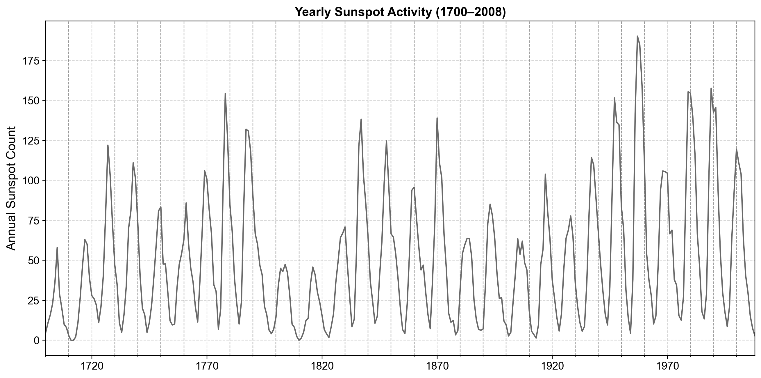
../_images/annual_sunspot_data.png — Fig. 4.15 Annual sunspot counts from 1700 to 2008, showing pronounced multi-year cycles in solar activity with varying peak intensity over time.#

Fig. 4.15 shows oscillatory behavior without an obvious linear trend, so we tentatively treat the series as stationary in mean after accounting for its stochastic structure. To confirm the type of dependence, we examine its autocorrelation functions:

../_images/sunspot_acf_pacf.png — Fig. 4.16 Sample ACF and PACF for annual sunspot counts, showing slowly decaying autocorrelations and several significant partial autocorrelations at low lags—patterns consistent with a low-order autoregressive structure rather than a pure moving-average process.#

The PACF shows significant autocorrelation at the first few lags before decaying, suggesting that a low-order AR model may be appropriate, while the ACF decays more gradually, which is consistent with AR(p) behavior rather than a pure MA(q) cut-off.

4.5.2.1. Fitting AR Models via ARIMA(p,0,0)#

We now fit AR(2) and AR(3) models, implemented as ARIMA with \(d=0\) and \(q=0\):

Dep. Variable: — AIC: 2622.637, BIC: 2637.570, HQIC: 2628.607
AR(2) parameters:

const      49.7462
ar.L1       1.3906
ar.L2      -0.6886
sigma2    274.7272
dtype: float64

Dep. Variable: — AIC: 2619.404, BIC: 2638.070, HQIC: 2626.867
AR(3) parameters:

const      49.7519
ar.L1       1.3008
ar.L2      -0.5081
ar.L3      -0.1296
sigma2    270.1011
dtype: float64

The AR(3) model achieves slightly lower AIC and BIC than AR(2), indicating a better fit despite the extra parameter. The estimated AR coefficients reflect the medium-term memory in the sunspot cycle—each year’s value depends on several previous years.

4.5.2.2. Residual Diagnostics#

A model is only acceptable if its residuals behave like white noise. We check this using residual plots, normality diagnostics, and autocorrelation of residuals:

Durbin-Watson statistic: 1.956

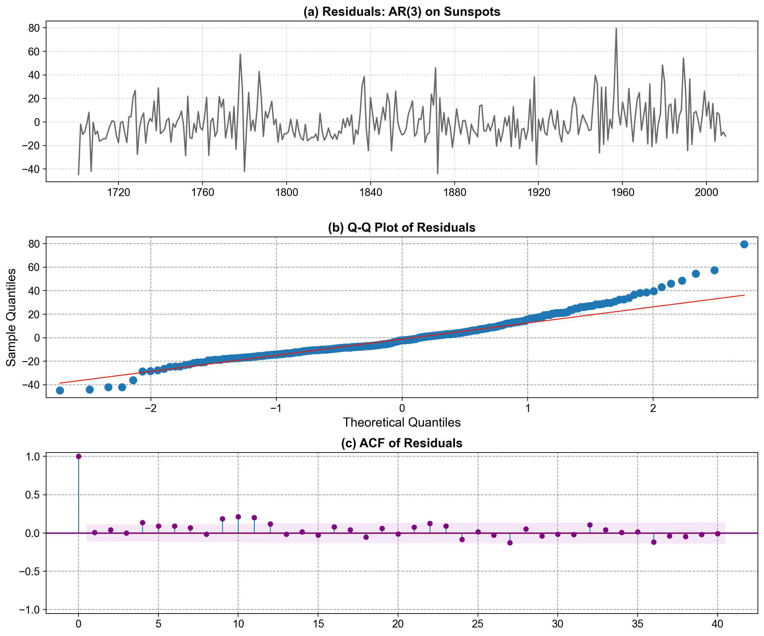
../_images/sunspot_arma30_resid_diagnostics.png — Fig. 4.17 Residual diagnostics for the AR(3) model fitted to annual sunspot counts. Panel **(a)** shows residuals fluctuating around zero without obvious long-term trends, suggesting that most large-scale structure in the series has been captured. Panel **(b)** presents a Q–Q plot comparing residual quantiles to a normal distribution; points follow the reference line closely in the center but deviate in the extreme tails, indicating only mild departures from normality. Panel **(c)** displays the ACF of the residuals, with most autocorrelations inside the confidence band, implying little remaining temporal dependence and supporting the adequacy of the AR(3) specification.#

After fitting the AR(3) model to the sunspot series, we use these diagnostics to check whether our model assumptions are reasonable. In Fig. 4.17, Panel (a) reassures us that residuals behave like noise rather than showing leftover trend or cyclic structure, which would indicate model underfitting. Panel (b) suggests that, for most quantiles, the Gaussian error assumption is acceptable for inference and prediction, even though extreme values are slightly heavier-tailed than a perfect normal distribution. Panel (c) shows that residual autocorrelations are small and mostly insignificant beyond lag 0, so the AR(3) model has successfully removed the main temporal dependence and leaves us with approximately white-noise errors, a key requirement for reliable ARMA/ARIMA forecasting.

The Durbin–Watson statistic of 1.956 is very close to 2, indicating minimal residual autocorrelation, and the residual ACF remains within the confidence bounds for nearly all lags, with only minor hints of remaining structure at longer lags. The Q–Q plot shows small deviations from normality in the tails, which is typical for real-world time series data. Taken together, these diagnostics suggest that the AR(3) model provides a reasonable stationary representation of the sunspot counts and serves as a clear example of ARMA-type modeling in the case \(d = 0\).

4.5.3. ARIMA on Non-Stationary Data: CPI Example#

We now turn to a series that clearly violates the stationarity assumption: U.S. quarterly CPI from 1959Q1 to 2009Q3. This series exhibits a strong upward trend, so an ARMA(p,q) model on the raw levels would be inappropriate.

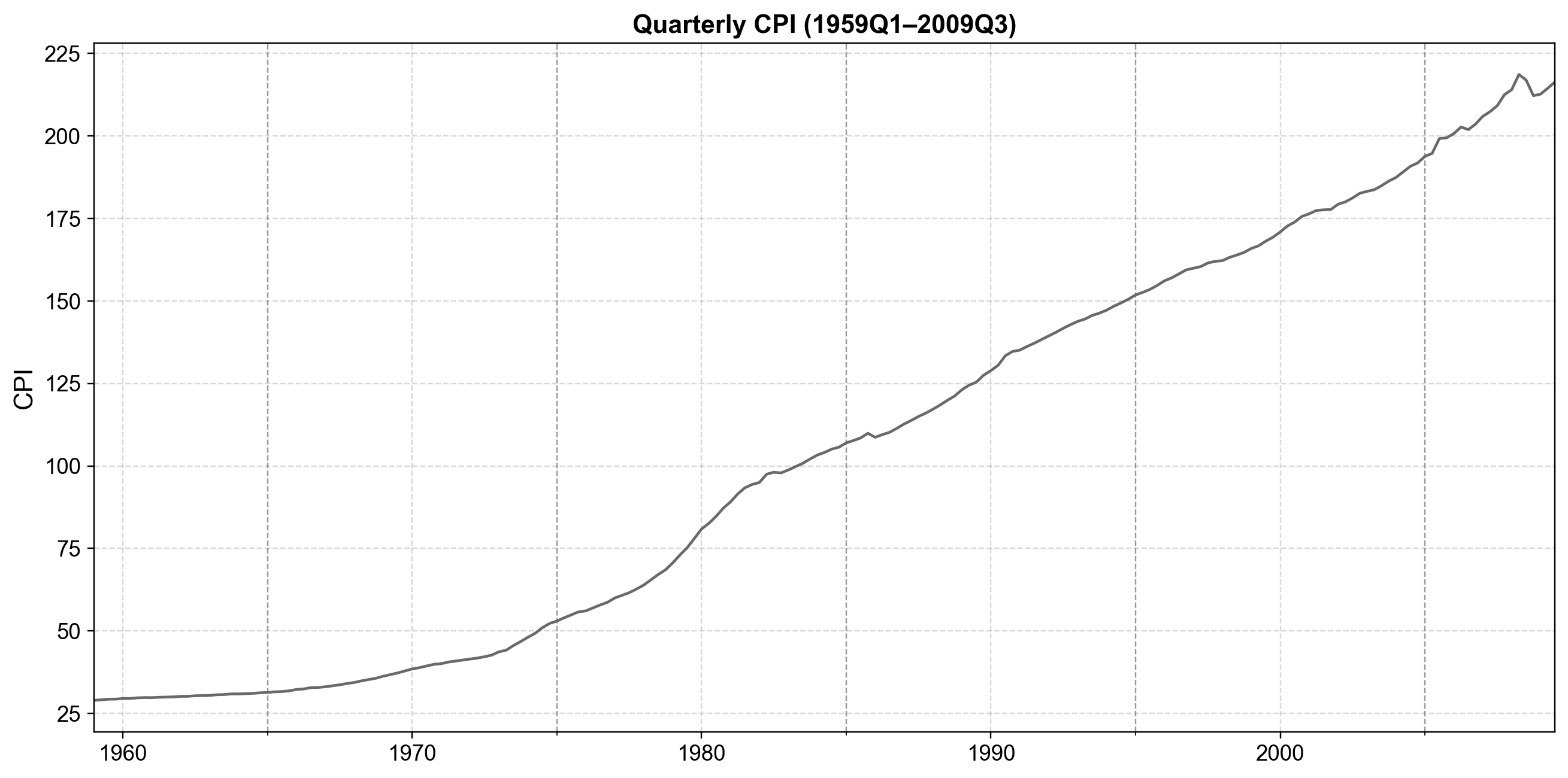
../_images/quarterly_cpi.png — Fig. 4.18 Quarterly U.S. Consumer Price Index (CPI) from 1959Q1 to 2009Q3, showing a persistent upward trend with no visible mean reversion—clear evidence of non-stationary behavior that motivates differencing before ARIMA modeling.#

Fig. 4.18 reveals a clear upward trajectory—CPI values do not fluctuate around a constant mean but increase persistently over time. To formalize this, we apply the Augmented Dickey–Fuller (ADF) test for a unit root:

ADF statistic on CPI levels: 0.7308
ADF p-value on CPI levels: 0.9904
Used lags: 12, observations: 190

The very high p-value (around 0.99) indicates that we cannot reject the null of a unit root, confirming that CPI levels are non-stationary. This is exactly the type of series for which ARIMA was designed.

4.5.3.1. Differencing and Stationarity#

We begin by taking the first difference to remove the linear trend:

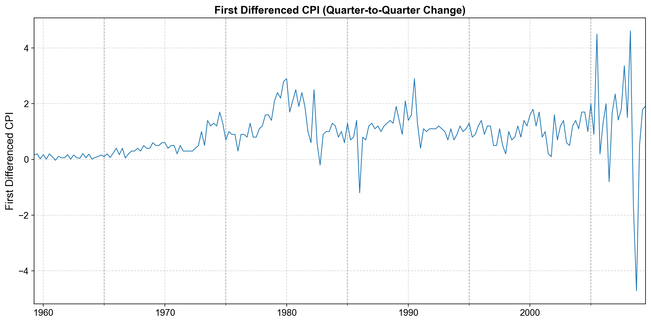
../_images/differenced_quarterly_cpi.png — Fig. 4.19 **First Difference (\(d=1\)).** Quarter-to-quarter changes in CPI. While the strong upward trend is gone, the series still shows signs of wandering behavior, particularly in the later years, suggesting that a single difference may not be enough to achieve full stationarity.#

ADF statistic (d=1): -2.7955
ADF p-value (d=1):   0.0589

The ADF test yields a p-value of 0.0589, which is slightly above the standard 0.05 significance threshold. This suggests the series is still borderline non-stationary.

To address this, we apply a second difference (i.e., the change in the change):

ADF statistic (d=2): -4.6675
ADF p-value (d=2):   0.0001

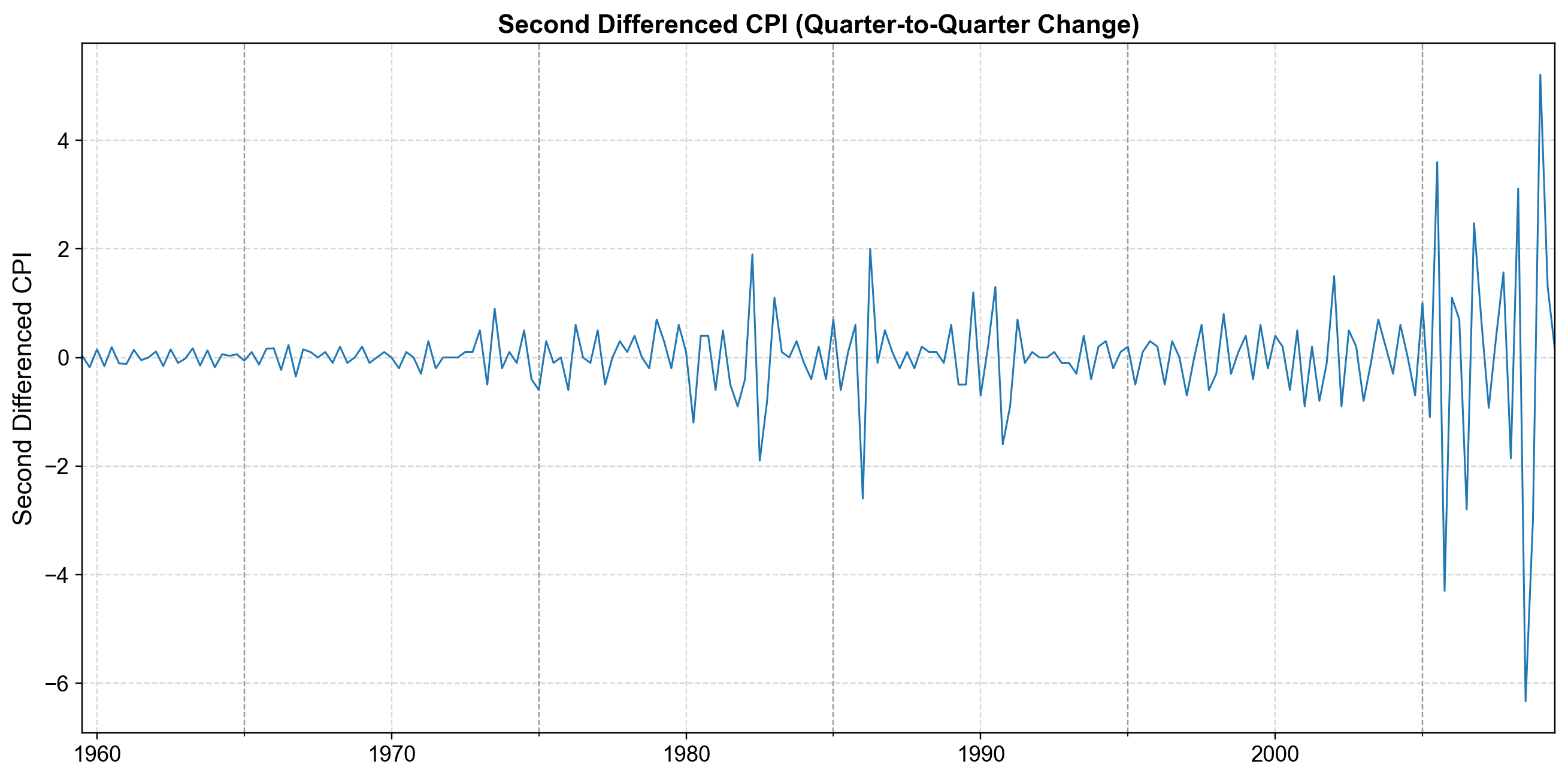
../_images/second_differenced_quarterly_cpi.png — Fig. 4.20 **Second Difference (\(d=2\)).** The acceleration of prices (change in inflation). This series oscillates rapidly around a constant mean of zero with stable variance. The ADF test confirms this is fully stationary (\(p < 0.01\)), identifying \(d=2\) as the appropriate differencing order for our ARIMA model.#

4.5.3.2. ACF/PACF on Second Differenced CPI#

Since we determined that \(d=2\) is required, we examine the ACF and PACF of the second differenced series (cpi_diff2) to identify the AR (\(p\)) and MA (\(q\)) orders.

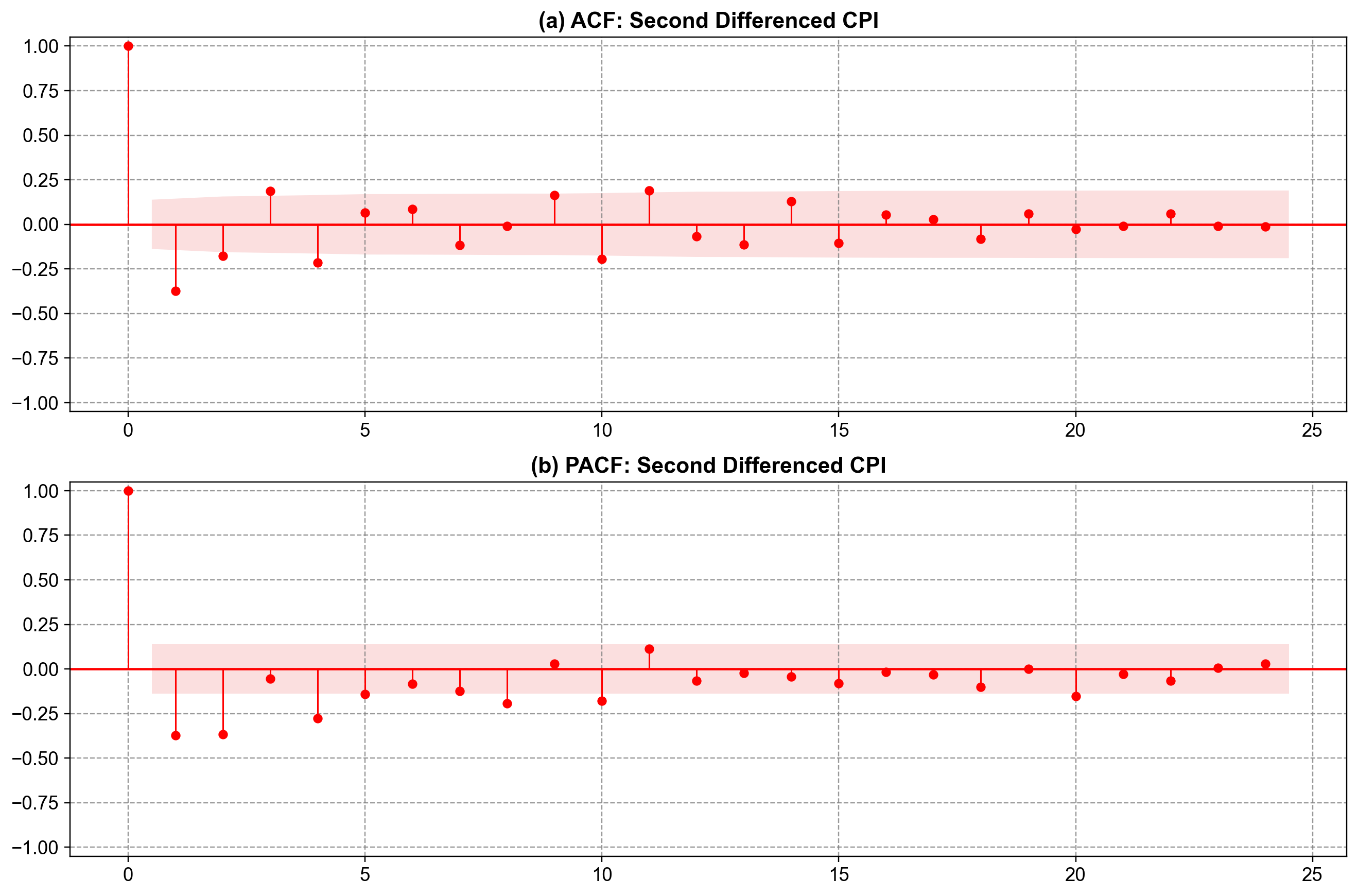
../_images/cpi_diff_second_acf_pacf.png — Fig. 4.21 Sample ACF and PACF of the **second differenced** CPI. **Panel (a):** The ACF shows a significant negative spike at Lag 1, followed by a sharp cutoff. This is the classic signature of an **MA(1)** process with a negative coefficient. **Panel (b):** The PACF shows a decaying or oscillating pattern (damped sine wave), which confirms the MA(1) diagnosis. **Conclusion:** The structure suggests an **ARIMA(0,2,1)** model.#

4.5.3.3. Fitting ARIMA Models (\(d=2\))#

Based on the ACF/PACF analysis, ARIMA(0,2,1) is our primary candidate. However, we will check neighbors like ARIMA(0,2,2) and ARIMA(1,2,1) to verify it is robust.

	AIC
ARIMA(0,2,2)	485.490740
ARIMA(1,2,1)	486.399113
ARIMA(0,2,1)	489.927914

The comparison table reveals that ARIMA(0,2,2) achieves the lowest AIC (485.49), slightly outperforming the simpler ARIMA(0,2,1) (489.93) and the ARIMA(1,2,1).

While the ACF plot showed a clear spike at lag 1 suggestive of an MA(1), the lower AIC for the MA(2) model implies that adding a second moving-average term captures additional residual structure that the simpler model misses. This result highlights the value of using Information Criteria (like AIC) alongside visual diagnostics: visual plots give us a starting point (MA(1)), but the quantitative metrics guide us to the optimal refinement (MA(2)).

4.5.3.4. Interpreting the ARIMA(0,2,1)#

The estimated model is:

\[\begin{equation*} \nabla^2 X_t = \varepsilon_t + \theta_1 \varepsilon_{t-1} \end{equation*}\]

Remark

Although ARIMA(0,2,2) had a slightly lower AIC, we examine the ARIMA(0,2,1) here as it is the more parsimonious candidate suggested by the ACF plots and serves as a clear baseline.

                               SARIMAX Results                                
==============================================================================
Dep. Variable:                    cpi   No. Observations:                  203
Model:                 ARIMA(0, 2, 1)   Log Likelihood                -242.964
Date:                Fri, 02 Jan 2026   AIC                            489.928
Time:                        12:14:13   BIC                            496.535
Sample:                    03-31-1959   HQIC                           492.601
                         - 09-30-2009                                         
Covariance Type:                  opg                                         
==============================================================================
                 coef    std err          z      P>|z|      [0.025      0.975]
------------------------------------------------------------------------------
ma.L1         -0.8497      0.028    -30.891      0.000      -0.904      -0.796
sigma2         0.6527      0.019     33.712      0.000       0.615       0.691
===================================================================================
Ljung-Box (L1) (Q):                   3.40   Jarque-Bera (JB):              4231.57
Prob(Q):                              0.07   Prob(JB):                         0.00
Heteroskedasticity (H):              23.57   Skew:                            -2.61
Prob(H) (two-sided):                  0.00   Kurtosis:                        24.86
===================================================================================

Warnings:
[1] Covariance matrix calculated using the outer product of gradients (complex-step).

The coefficient \(\theta_1 \approx -0.85\) is highly significant (\(P < 0.001\)) and negative. A negative MA parameter in a differenced series is very common; it acts as a “correction” mechanism. It implies that if the acceleration of prices “overshoots” in one quarter (a large positive shock), the model expects a partial reversal (a negative contribution) in the next quarter’s acceleration. This negative correlation helps stabilize the second-differenced series, keeping it stationary around zero.

4.5.3.5. Forecasting with ARIMA#

To illustrate forecasting, we split the CPI data into training (first 85%) and test (last 15%) sets. We then fit our chosen ARIMA(0,2,1) model to the training data and project it forward.

We plot the results to visually assess the model’s performance:

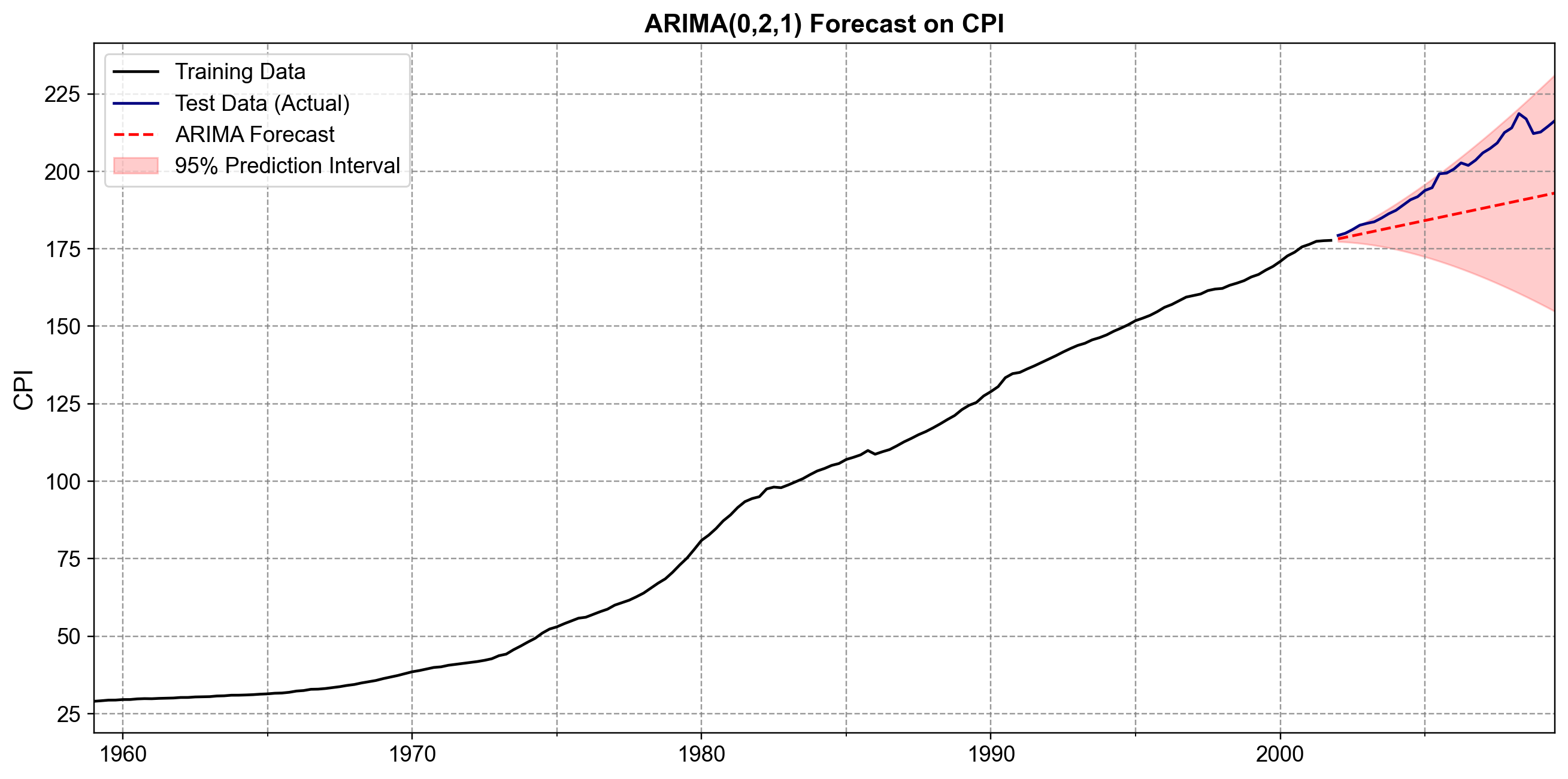
../_images/cpi_arima_forecast.png — Fig. 4.22 **Forecasting with ARIMA(0,2,1).** The black curve shows the training data, the navy curve shows the actual held-out observations, and the red dashed line is the forecast. Because the model uses \(d=2\) (second differencing), it projects a linear trend based on the most recent “velocity” (change in inflation) at the end of the training set. The 95% prediction interval (red shaded region) widens rapidly, correctly reflecting the high uncertainty of predicting non-stationary macroeconomic data over long horizons.#

Finally, we compute quantitative accuracy metrics on the test set:

Test RMSE: 15.371
Test MAE:  13.005

The test RMSE of 15.371 indicates a reasonably strong fit, especially compared to simpler trend models. The ARIMA(0,2,1) model successfully captured the local “velocity” of inflation at the end of the training period and projected it forward. Because \(d=2\) implies a flexible trend (allowing for acceleration/deceleration), the model was able to adapt to the changing slope of the CPI curve better than a linear trend model (\(d=1\)) would have.

This completes a full ARIMA workflow on a trending macroeconomic series using standard statsmodels datasets and APIs.

Summary

Sunspots (Stationary): We used an AR(2) (or ARIMA(2,0,0)) because the data was effectively stationary. The workflow focused on capturing the periodic cycle.
CPI (Non-Stationary): We used an ARIMA(0,2,1) because the data exhibited a non-linear trend. The workflow required:
1. Stationarity Testing: Using the ADF test to determine that second differencing (\(d=2\)) was necessary to achieve stationarity.
2. Order Selection: Using ACF/PACF on the second-differenced data to identify an MA(1) signature.
3. Forecasting: Projecting the acceleration of prices forward, resulting in a robust forecast with appropriate uncertainty bounds.

In the next section, we will extend these ideas to Seasonal ARIMA (SARIMA) models, which add seasonal AR, MA, and differencing components to handle recurring patterns such as yearly cycles in monthly data.