Remark
Please be aware that these lecture notes are accessible online in an ‘early access’ format. They are actively being developed, and certain sections will be further enriched to provide a comprehensive understanding of the subject matter.
3.1. Understanding Seasonality#
Seasonality refers to predictable, recurring patterns in time series data that occur at regular intervals. These patterns are driven by calendar-related factors such as seasons, months, weeks, or specific events like holidays. Unlike irregular fluctuations or random noise, seasonal patterns repeat consistently over time, making them valuable for forecasting and business planning [Davey and Flores, 1993].
3.1.1. Types of Seasonal Patterns#
Seasonal patterns manifest at regular calendar intervals and are shaped by weather, holidays, cultural events, scheduling cycles, and customer behavior. The examples below pair realistic use cases with illustrative synthetic data.
3.1.1.1. Annual Seasonality#
Annual effects recur each year, with consistent timing and varying intensity depending on the product’s seasonality.
Example 3.1 (Synthetic Data Examples)
Clothing Sales (Winter Peak): Retail apparel shows strong winter seasonality, peaking at $70,324 in January and bottoming at $30,116 in July (≈2.3× peak-to-trough), reflecting cold-weather demand and holiday shopping cycles.
Ice Cream Sales (Summer Peak): Ice cream sales peak at $48,843 in July and drop to $10,503 in February (≈4.7×), characteristic of temperature-sensitive categories.
Heating Costs (Winter Peak): Heating expenditures reach $363 in winter and fall to $152 in summer (≈2.4×), driven by thermal load and fuel use.
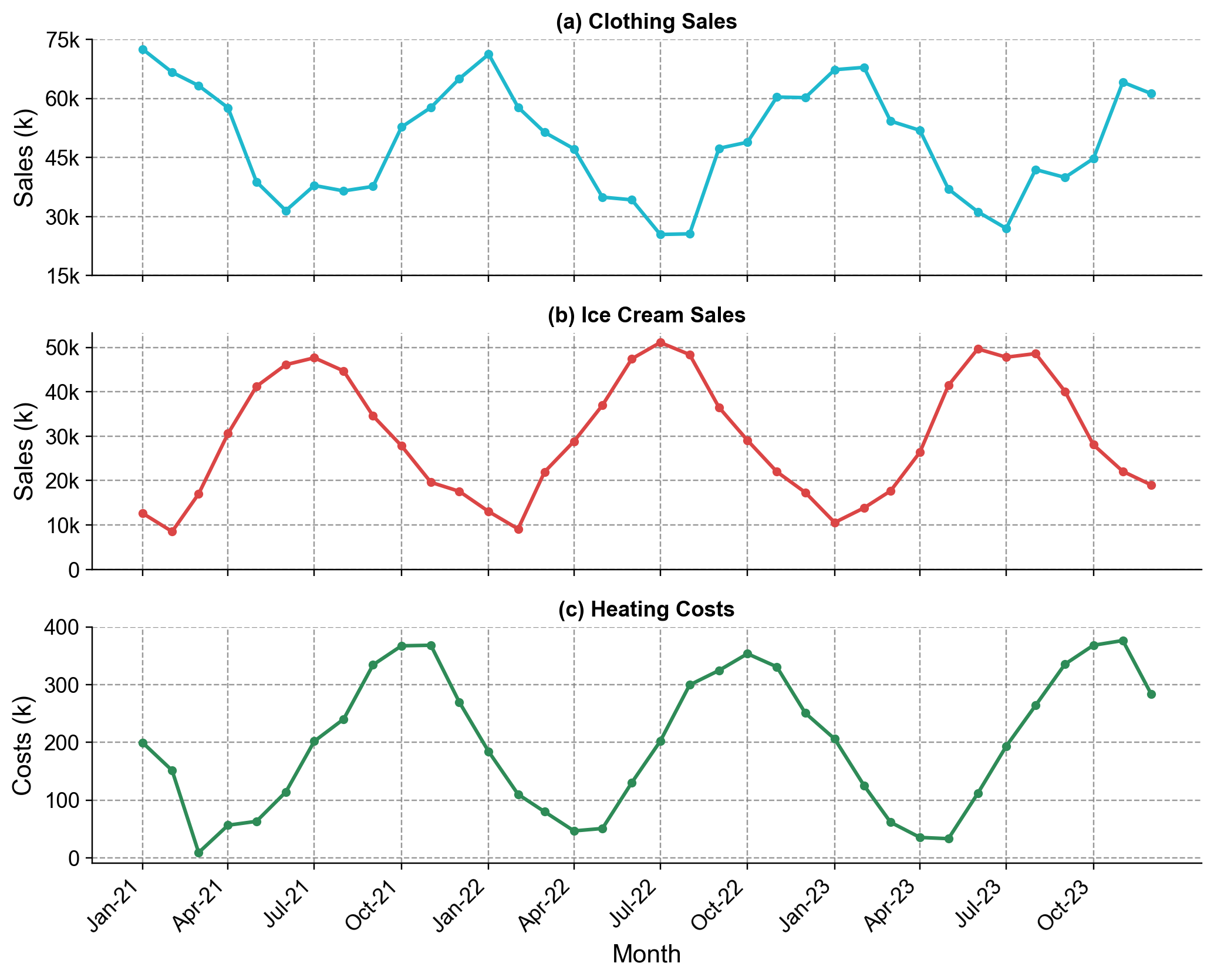
Fig. 3.1 Three annual seasonal profiles: winter-peaking clothing sales, summer-peaking ice cream sales, and winter-peaking heating costs.#
(a) Clothing Sales (Winter Peak): Peaks at $70,324 in January, lows at $30,116 in July (≈2.3×), driven by seasonal apparel demand and holiday cycles.
(b) Ice Cream Sales (Summer Peak): Peaks at $48,843 in July, lows at $10,503 in February (≈4.7×), illustrating temperature-driven demand.
(c) Heating Costs (Winter Peak): Peaks at $363 in winter, lows at $152 in summer (≈2.4×), reflecting seasonal energy consumption.
3.1.1.2. Monthly Seasonality#
Monthly patterns occur within calendar months and are often related to billing cycles, payroll schedules, or monthly business processes.
Example 3.2 (Synthetic Data Examples)
Credit Card Payments (Salary Date Effects): Payment volumes peak on days 28-2 of each month with averages of $25,288 on day 29 and $25,242 on day 1. This pattern reflects typical bi-monthly payroll schedules where employees receive salaries at month-end and mid-month, creating a 1.7x amplitude difference between peak and low payment days.
Utility Bill Payments: Utility payments show concentrated spikes during billing periods, particularly days 7-9 of each month, with peak payments reaching $8,151 on day 7. This creates an extreme 16.5x amplitude difference, as most customers pay within a narrow window after receiving bills.
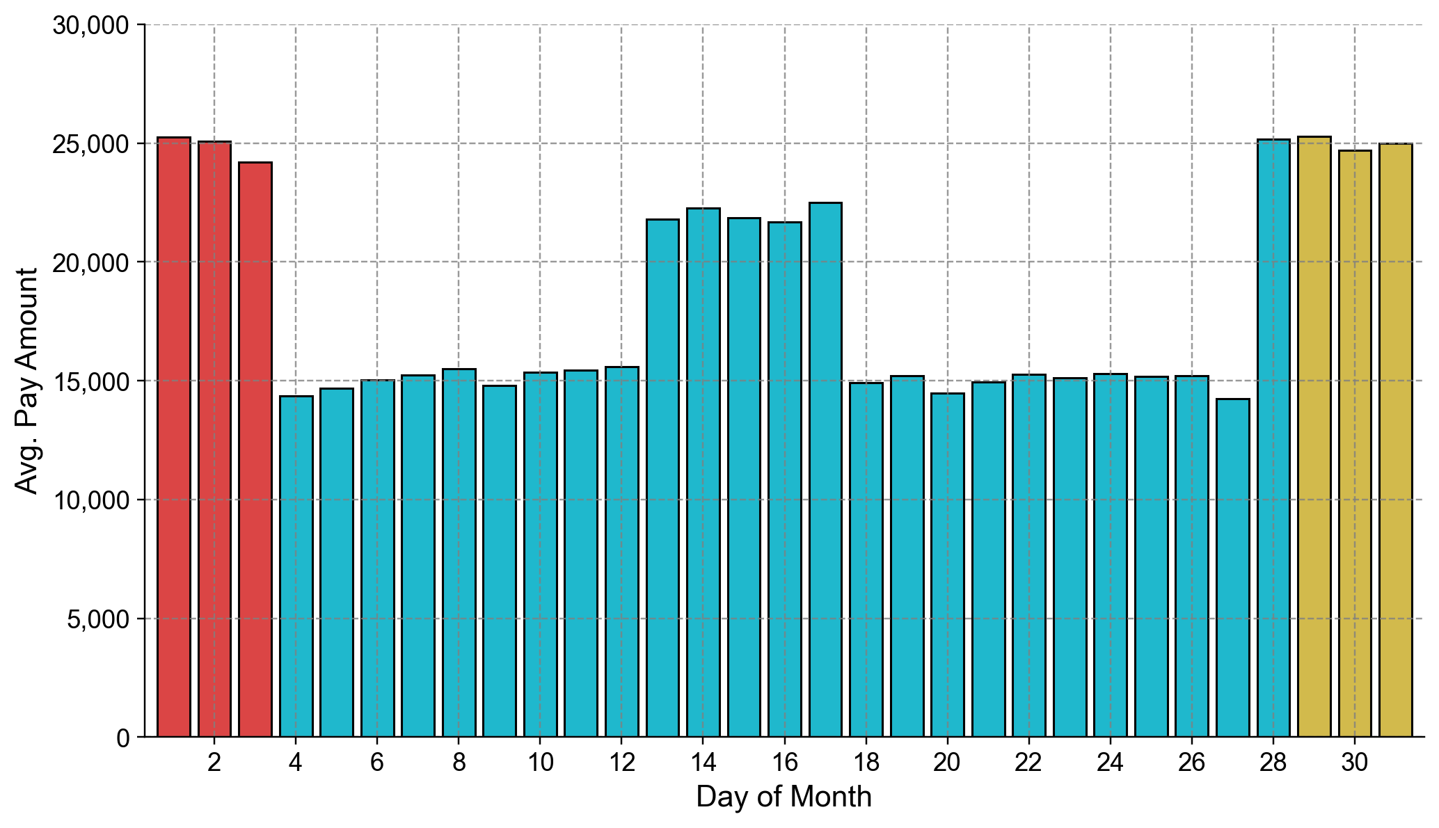
Fig. 3.2 Monthly seasonality showing credit card payment spikes at month-end and month-beginning, corresponding to typical salary payment dates#
3.1.1.3. Weekly Seasonality#
Weekly patterns reflect differences between weekdays and weekends, driven by work schedules, leisure activities, and business operations.
Example 3.3 (Synthetic Data Examples)
Website Traffic (Business Day Pattern): Website traffic shows consistent weekday patterns with Monday-Friday averaging 640-657 visitors per hour, while weekends drop to 372-388 visitors per hour. This 1.8x amplitude reflects B2B website usage patterns where business activity drives traffic.
Restaurant Sales (Weekend Pattern): Restaurant sales demonstrate strong weekend seasonality, with Saturday-Sunday averaging $803-804 per hour compared to Monday-Friday at $290-335 per hour. This 2.8x weekend premium reflects leisure dining patterns and social activities concentrated on weekends.
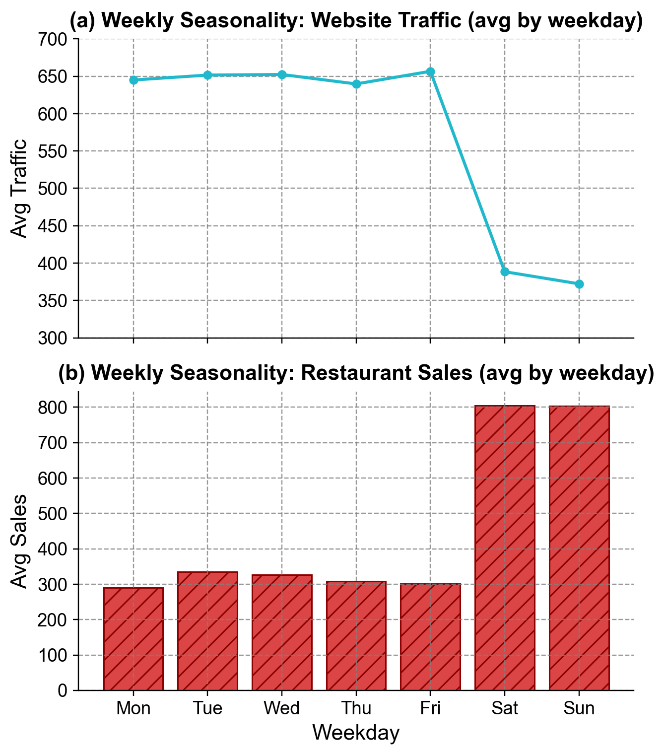
Fig. 3.3 (a) Weekly Seasonality: Website Traffic (avg by weekday). Weekday traffic is consistently higher (Mon–Fri ≈ 640–657 visits/hour) than weekends (Sat–Sun ≈ 372–388 visits/hour), yielding ≈1.8× weekday-to-weekend amplitude typical of B2B usage patterns.#
(b) Weekly Seasonality: Restaurant Sales (avg by weekday). Weekend sales surge (Sat–Sun ≈ $803–$804/hour) relative to weekdays (Mon–Fri ≈ $290–$335/hour), a ≈2.8× weekend premium reflecting leisure dining and social activity concentration.
3.1.1.4. Daily Seasonality#
Daily patterns show variations within 24-hour periods, typically reflecting business hours, peak usage times, or natural activity cycles.
Example 3.4 (Synthetic Data Examples)
Call Center Volume (Business Hours Pattern): Call center volume peaks during business hours, with maximum activity at 3:00 PM (157 calls/hour) and minimum activity during overnight hours (20 calls/hour). This creates a 7.9x amplitude difference, clearly showing the business hours constraint on customer service demand.
Energy Consumption (Peak Load Pattern): Energy consumption shows dual peaks during morning (6-9 AM) and evening (6-10 PM) periods, with evening peaks reaching 96 units/hour and overnight lows of 45 units/hour. This 2.1x daily amplitude reflects residential and commercial activity patterns.
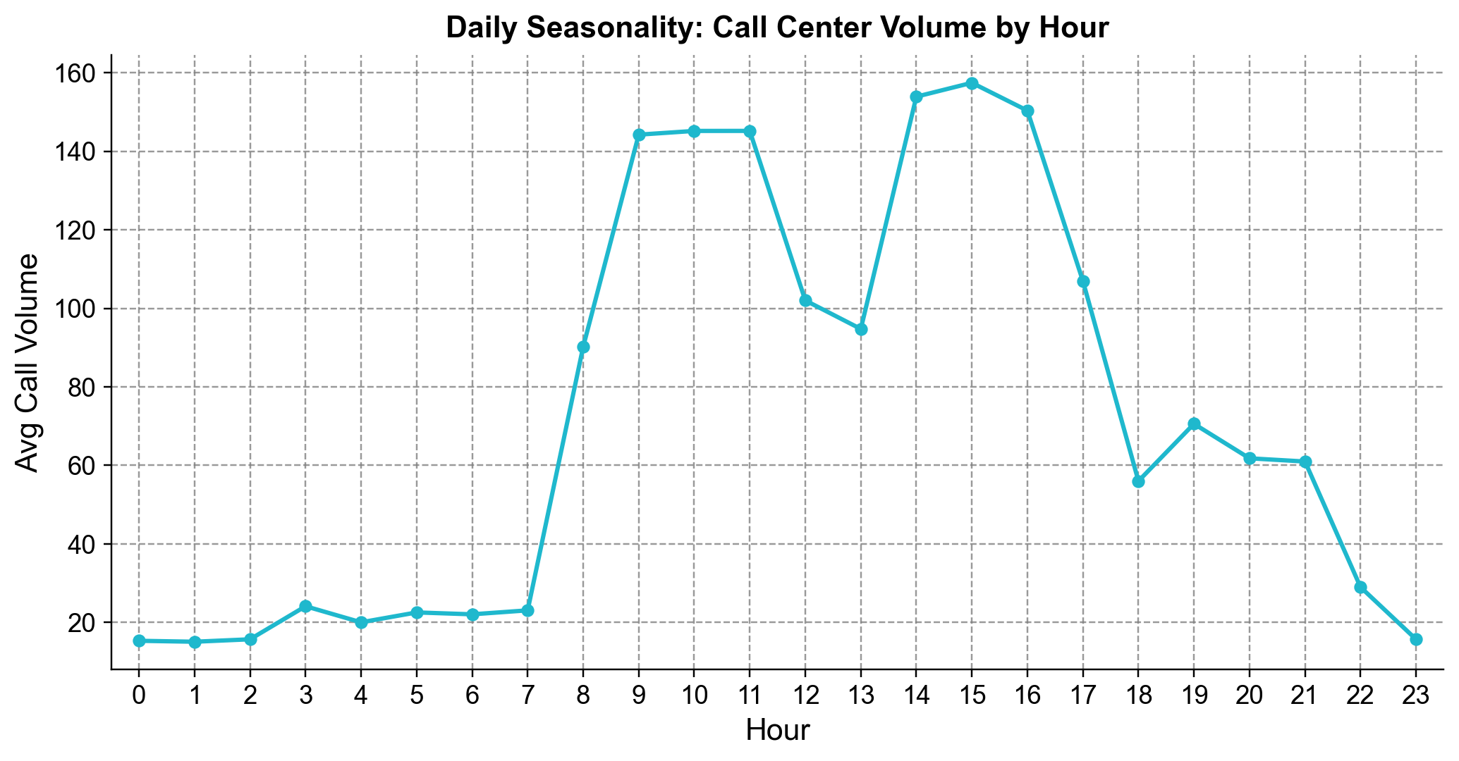
Fig. 3.4 Daily seasonality pattern showing call center volume peaks during business hours (9 AM - 5 PM) with lower activity during evening and night hours#
3.1.1.5. Holiday Effects#
Holiday effects are irregular but predictable patterns around specific dates, creating dramatic spikes or dips that don’t follow regular calendar cycles.
Example 3.5 (Synthetic Data Examples)
E-commerce Sales (Shopping Holiday Effects): The analysis reveals extreme holiday seasonality with Black Friday period sales averaging $282,480 per day and Christmas period sales at $283,487 per day, compared to a baseline of $102,140 per day. This represents a 176.6% uplift during peak shopping periods, followed by a post-holiday drop in January to $60,520 per day (-40.7% below baseline).
Travel Bookings (Seasonal Planning Cycles): Travel bookings show advance booking patterns with peaks during March-May (2.0x multiplier) for summer travel planning and September-November (1.7x multiplier) for winter vacation bookings. January shows a dramatic 60% drop as consumers recover from holiday spending.
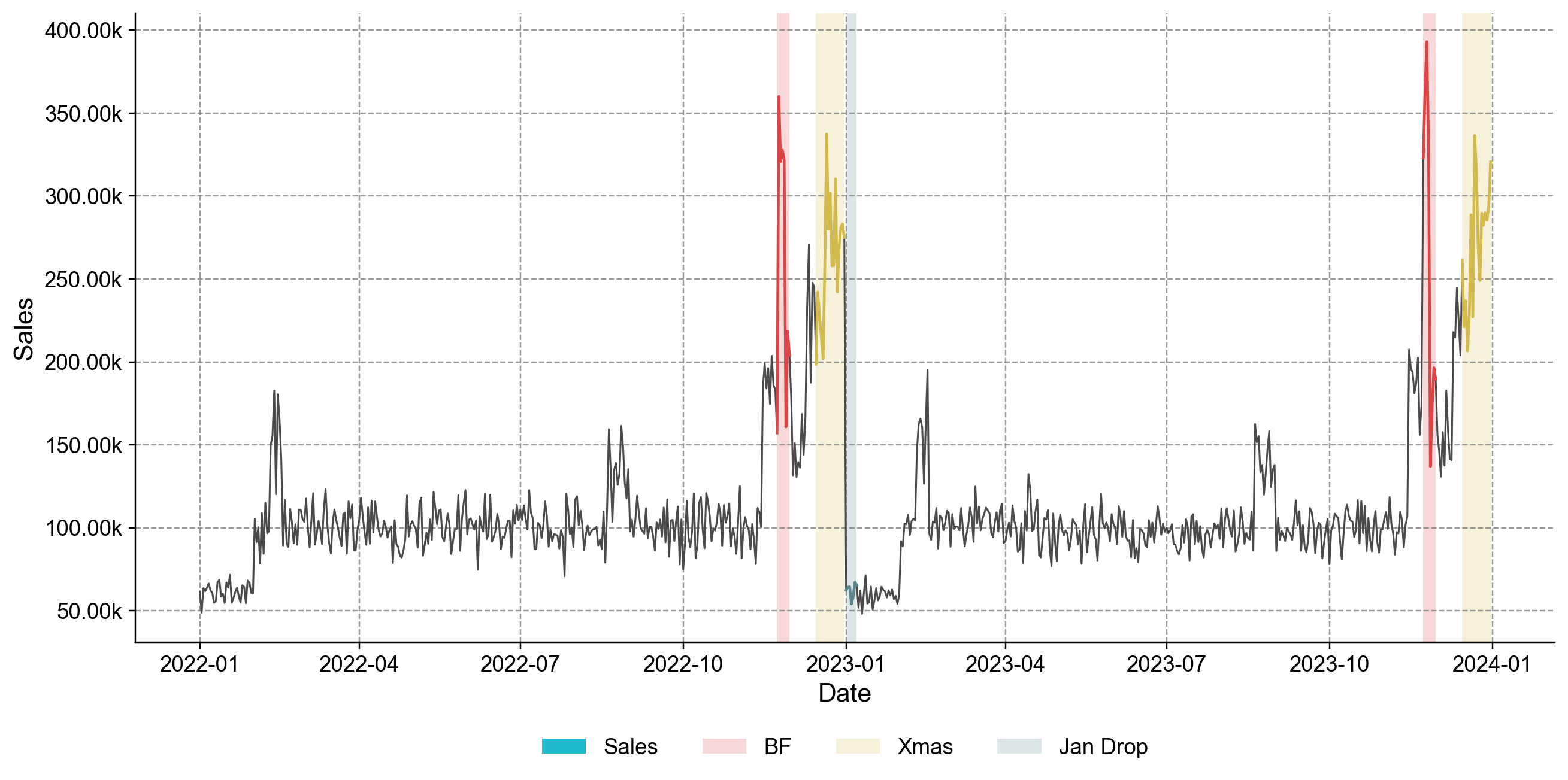
Fig. 3.5 Holiday Effects in E‑commerce Sales. Daily sales exhibit irregular but predictable holiday-driven spikes: Black Friday period averages ≈ $282,480/day and the Christmas period ≈ $283,487/day, versus a baseline of ≈ $102,140/day (≈ +176.6%), followed by a January post‑holiday drop to ≈ $60,520/day (≈ −40.7%). Travel demand shows complementary planning cycles with advance booking surges in Mar–May (≈2.0×) for summer trips and Sep–Nov (≈1.7×) for winter vacations, with January booking volumes dipping sharply as consumers normalize post‑holidays.#
3.1.2. Mathematical Framework#
Time series with seasonality can be modeled using two main approaches:
Additive Model:
In additive models, seasonal fluctuations remain constant over time regardless of the overall level of the series.
Multiplicative Model:
In multiplicative models, seasonal effects scale proportionally with the trend, making them more appropriate for data where seasonal variations increase or decrease with the overall level.