Remark
Please be aware that these lecture notes are accessible online in an ‘early access’ format. They are actively being developed, and certain sections will be further enriched to provide a comprehensive understanding of the subject matter.
5.5. Descriptive Statistics-Based Methods for Outlier Detection in Time Series#
5.5.1. Z-Score Method#
The Z-score method provides a standardized measure of how far an observation deviates from the dataset mean, expressed in units of standard deviation. This transformation creates a scale-free metric that allows comparison across different measurement units and facilitates threshold-based outlier detection [Leys et al., 2013].
Formula:
where \(x\) represents the observation, \(\mu\) is the sample mean, and \(\sigma\) is the sample standard deviation.
Decision Rule: Flag observations where \(|Z| > 3\) as potential outliers. This threshold corresponds to values more than three standard deviations from the mean, which under a normal distribution would occur with probability less than 0.3%.
Example 5.4
Consider daily temperature measurements with mean \(\mu = 72.5°F\) and standard deviation \(\sigma = 8.7°F\):
A reading of 104°F yields: \(Z = \dfrac{104-72.5}{8.7} = 3.62\) → Outlier (exceeds threshold)
A reading of 85°F yields: \(Z = \dfrac{85-72.5}{8.7} = 1.44\) → Normal variation
A reading of 98°F yields: \(Z = \dfrac{98-72.5}{8.7} = 2.93\) → Normal (below threshold, though elevated)
The 104°F reading exceeds the \(|Z| > 3\) criterion, indicating it is substantially more extreme than typical daily variation and warrants investigation for potential sensor malfunction or genuine weather anomaly.
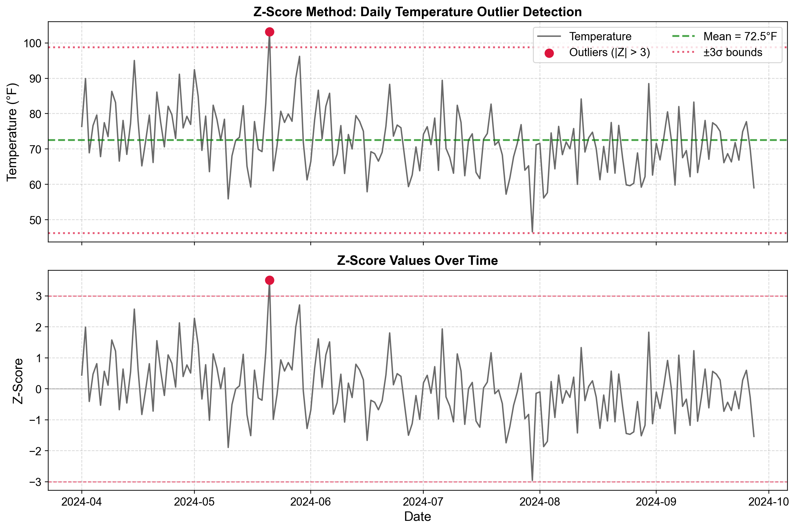
Fig. 5.24 Z-score method applied to daily temperature data. The top panel shows raw temperatures with mean (72.5°F) and ±3σ control bounds (approximately 46°F and 99°F). The bottom panel displays standardized z-scores with threshold lines at ±3, revealing one observation exceeding the upper limit.#
Fig. 5.24 demonstrates the Z-score method applied to temperature measurements collected from April through September 2024. The top panel displays the original temperature series with the mean indicated by the green dashed line at 72.5°F. Red dotted lines mark the ±3σ bounds at approximately 46°F and 99°F. One observation in late May reaches approximately 104°F, appearing as a clear spike above the upper control limit and marked with a red circle.
The bottom panel transforms these same observations into z-scores, creating a standardized view where the mean becomes zero and the scale represents standard deviations. Most observations fluctuate between -2 and +2, indicating typical variation within two standard deviations of the mean. The same late May observation now appears at approximately z = 3.6, clearly exceeding the red threshold line at z = +3. This transformation makes the outlier’s statistical extremity immediately apparent—it is not merely “hot” but specifically 3.6 times more extreme than the typical variation pattern.
Sensitivity to Contamination: The Z-score method suffers from a critical weakness known as masking. Because both \(\mu\) and \(\sigma\) are calculated from the data, extreme outliers inflate the standard deviation and shift the mean toward themselves. This reduces their own z-scores, potentially preventing detection. For example, if the dataset contains several extreme high values, \(\sigma\) increases and \(\mu\) shifts upward, making those extreme values appear less unusual than they actually are.
Distributional Assumptions: The \(|Z| > 3\) threshold assumes data follow an approximately normal distribution. For heavy-tailed or skewed distributions, this threshold may be too conservative (missing legitimate outliers) or too liberal (flagging natural variation). The method performs poorly on asymmetric data where extreme values occur more frequently in one direction.
Global Perspective Only: Z-scores are calculated using global mean and standard deviation, making them ineffective for contextual outliers. A temperature of 75°F might yield a modest z-score when computed across an entire year, yet represent a clear anomaly for January. For seasonal data, compute separate z-scores within each seasonal group rather than using global statistics.
5.5.2. Modified Z-Score Method#
The Modified Z-Score method addresses the primary weakness of the standard Z-score: sensitivity to the outliers it is trying to detect. By replacing the mean with the median and the standard deviation with the Median Absolute Deviation (MAD), the method achieves robustness—extreme values have minimal influence on the location and scale estimates used for detection [Huber and Ronchetti, 2009].
Formula:
where \(\tilde{x}\) is the sample median, \(MAD = \text{median}(|x_i - \tilde{x}|)\), and the constant 0.6745 converts MAD to an estimate of the standard deviation under normality.
Decision Rule: Flag observations where \(|M| > 3.5\) as potential outliers. The slightly higher threshold compared to the standard Z-score (3.5 versus 3.0) accounts for the different statistical properties of MAD-based estimates.
Example 5.5
Consider monthly sales data with median \(\tilde{x} = \$108,900\) and \(MAD = \$32,400\):
Sales of $155,000: \(M = \dfrac{0.6745(155000-108900)}{32400} = 0.96\) → Normal variation
Sales of $240,000: \(M = \dfrac{0.6745(240000-108900)}{32400} = 2.73\) → Elevated but acceptable
Sales of $495,000: \(M = \dfrac{0.6745(495000-108900)}{32400} = 8.03\) → Clear outlier
The $495,000 month substantially exceeds the \(|M| > 3.5\) threshold, indicating performance dramatically beyond typical variation that requires investigation for either exceptional business success or data quality issues.
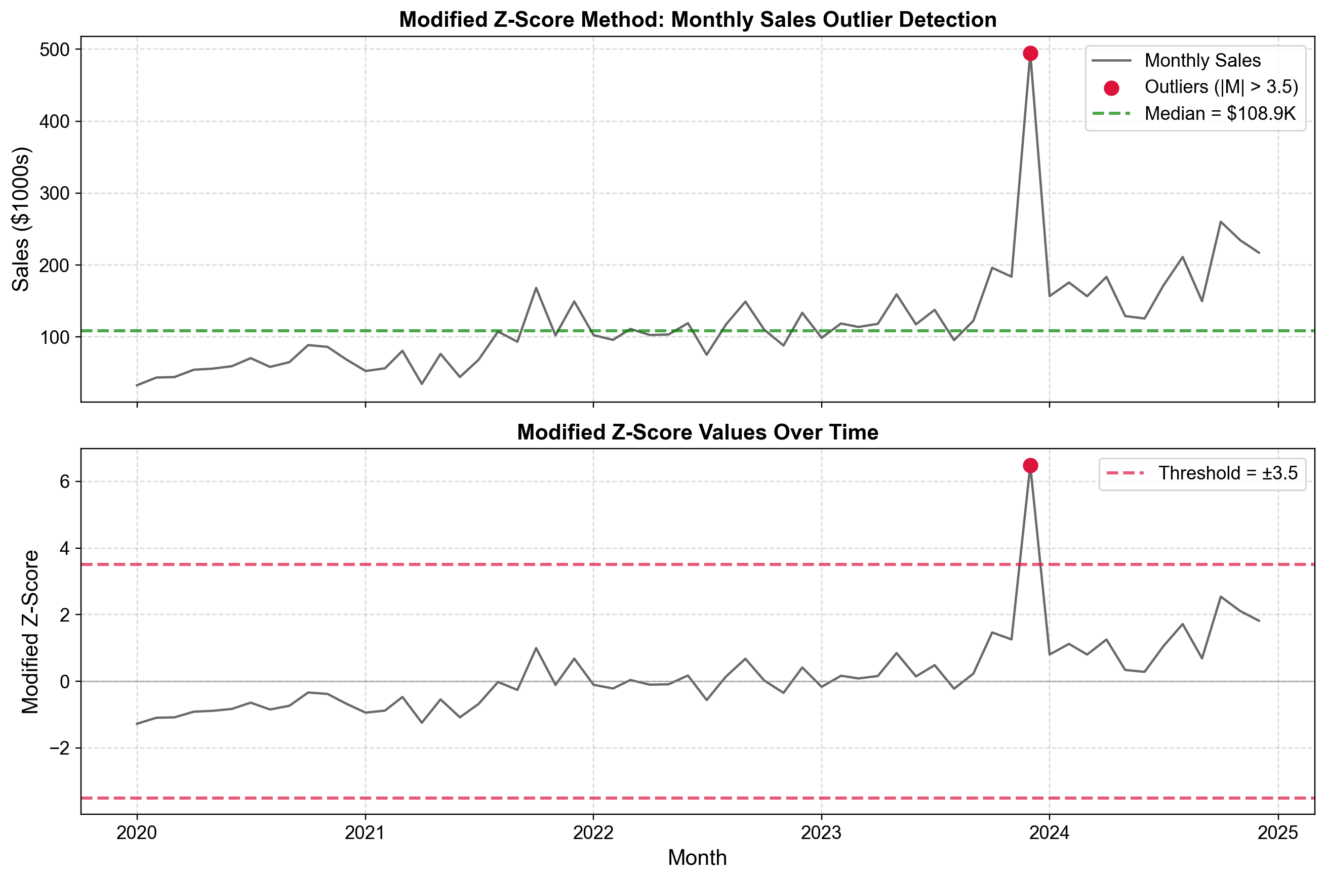
Fig. 5.25 Modified Z-Score method applied to monthly sales data spanning 2020-2025. The robust method uses median ($108.9K) and MAD, successfully identifying an extreme sales spike in mid-2024 that reaches approximately $495K with a modified z-score exceeding 6.#
Fig. 5.25 demonstrates the Modified Z-Score method applied to monthly sales data collected from January 2020 through late 2025. The top panel displays the original sales time series showing an overall upward trend from approximately $40,000 in early 2020 to fluctuations around $150,000-$250,000 by 2024-2025. The green dashed line marks the median at $108,900, representing the central tendency across the entire period. Most observations cluster between $50,000 and $250,000, reflecting typical monthly variation and the long-term growth trend.
A dramatic spike appears in mid-2024, reaching approximately $495,000—marked with a red circle as a detected outlier. This value stands approximately 4.5 times higher than the median, representing an extraordinary deviation from typical performance. Unlike the standard Z-score method where such an extreme value would inflate the mean and standard deviation (potentially masking itself), the Modified Z-Score’s use of median and MAD ensures robust detection regardless of the outlier’s magnitude.
The bottom panel transforms the same sales data into Modified Z-scores, creating a scale where the median becomes zero and deviations are measured in robust scale units. Most observations fluctuate between -1 and +2, indicating typical variation within expected bounds. The mid-2024 outlier now appears at approximately \(M = 6.3\), dramatically exceeding the red threshold line at \(M = 3.5\). This makes the statistical extremity immediately apparent—the observation is not merely “high sales” but specifically more than 6 robust standard deviations above the median.
The upward trend visible in the sales data (higher values in 2024-2025 compared to 2020-2021) does not substantially affect the Modified Z-score calculations because the median captures the central tendency across all periods. However, for data with strong temporal trends, detrending before applying the Modified Z-Score method may improve detection accuracy by focusing on deviations from expected trajectory rather than deviations from overall median.
Robustness to Contamination: The median has a breakdown point of 50%, meaning up to half the data can be outliers before the estimate becomes unreliable. MAD similarly resists contamination. In contrast, the mean and standard deviation have breakdown points near 0%, making them extremely sensitive to even a single outlier. This robustness is critical when outliers may be present but undetected in initial screening.
Performance with Skewed Distributions: For asymmetric distributions, the median provides a better measure of central tendency than the mean, which is pulled toward the longer tail. MAD similarly provides a more appropriate scale measure than standard deviation for non-normal data. The Modified Z-Score therefore performs better on the heavy-tailed and skewed distributions common in financial, environmental, and operational data.
Interpretability: Despite using robust statistics, Modified Z-scores maintain similar interpretation to standard Z-scores—they measure standardized distance from center. The 3.5 threshold corresponds roughly to the same tail probability as the 3.0 threshold for standard Z-scores under normality, maintaining consistent decision rules across methods.
Threshold Selection: While 3.5 is the standard threshold, applications requiring higher sensitivity to outliers may use 3.0, while those prioritizing specificity may use 4.0 or higher. The choice should reflect the relative costs of false positives (investigating normal variation) versus false negatives (missing genuine anomalies).
Computational Efficiency: Computing medians and MAD requires sorting operations, making the Modified Z-Score computationally slower than the standard Z-score for very large datasets. However, for typical time series with thousands to millions of observations, modern computing makes this difference negligible.
Temporal Patterns: Like the standard Z-score, the Modified Z-Score operates globally across all time periods. For data with strong trends, seasonality, or regime changes, consider applying the method within homogeneous segments (seasons, operational modes) rather than to the entire series at once.
5.5.3. Interquartile Range (IQR) Method#
The Interquartile Range method provides a distribution-free approach to outlier detection that relies on quartiles rather than moments. This makes it substantially more robust than Z-score methods when data contain contamination or depart from normality. The IQR method forms the statistical foundation for box plot outlier detection, one of the most widely used visual tools in exploratory data analysis [Dawson, 2011, Schwertman et al., 2004].
Method: Calculate the first quartile \(Q1\) (25th percentile) and third quartile \(Q3\) (75th percentile), then define:
The outlier detection boundaries are:
Decision Rule: Flag any observation falling below the lower bound or above the upper bound as a potential outlier.
Example 5.6
Consider hourly website traffic with \(Q1 = 1,076\) visitors, \(Q3 = 1,858\) visitors:
\(IQR = 1,858 - 1,076 = 782\) visitors
Lower bound: \(1,076 - 1.5(782) = -97\) visitors (effectively 0, since traffic cannot be negative)
Upper bound: \(1,858 + 1.5(782) = 3,031\) visitors
Traffic volumes of 2,850 visitors would be considered normal (below upper bound), while 3,500 visitors would be flagged as an outlier requiring investigation for potential causes such as viral content, bot traffic, or marketing campaign success.

Fig. 5.26 IQR method applied to hourly website traffic over a three-week period. Global IQR bounds (top panel) identify extreme spikes, while hour-specific analysis (bottom panel) reveals contextual outliers that deviate from typical patterns for specific times of day.#
Fig. 5.26 demonstrate the IQR method applied to hourly website traffic data collected continuously over approximately three weeks in May 2024. The top panel displays the time series with horizontal reference lines marking the IQR-based detection boundaries. Traffic typically ranges between 700 and 2,300 visitors per hour, with \(Q1 = 1,076\) and \(Q3 = 1,858\) calculated across all observations. The upper bound at 3,031 visitors (shown as a red dashed line) represents the threshold beyond which observations are flagged as outliers. One prominent spike on May 9 at 8:00 AM reaches approximately 2,849 visitors—just below the threshold—while any traffic exceeding 3,031 would be marked as a clear outlier.
The bottom panel would group traffic by hour of day, creating 24 separate box plots that reveal diurnal patterns. This contextual view exposes important structure: late-night hours (2:00-6:00 AM) typically see 900-1,400 visitors with correspondingly lower IQR-based thresholds, while evening peak hours (7:00-10:00 PM) regularly reach 1,800-2,200 visitors with higher thresholds. An observation of 2,000 visitors at 3:00 AM would appear as a severe outlier (far exceeding typical late-night traffic), even though the same 2,000 visitors at 9:00 PM falls well within normal variation. This hour-specific analysis demonstrates a critical principle: outlier detection should respect temporal context rather than applying global thresholds blindly.
Robustness to Contamination: Quartiles have a breakdown point of 25%, meaning up to one-quarter of the data can be outliers without substantially affecting \(Q1\) and \(Q3\) estimates. This provides much greater resistance to contamination than mean-based methods, which can be severely distorted by even a single extreme value.
Distribution-Free Application: The IQR method requires no assumptions about the underlying distribution. It performs reliably on skewed, heavy-tailed, or multimodal data where parametric methods fail. For symmetric distributions like the normal, approximately 0.7% of observations fall beyond the 1.5 × IQR fences, but the method adapts automatically to asymmetric distributions without requiring transformation.
Intuitive Interpretation: The method’s logic is transparent—outliers are observations that fall far from the central 50% of the data, where “far” is defined relative to the width of that central region. This makes results easy to explain to non-statistical audiences compared to methods requiring understanding of standard deviations or probability distributions.
Visual Integration: The IQR method directly corresponds to box plot construction, where whiskers extend to the outlier boundaries and individual points beyond whiskers are automatically flagged. This tight connection between numerical detection and visual inspection facilitates exploratory analysis and communication of findings.
Threshold Variations: While 1.5 × IQR represents the standard “inner fence” proposed by Tukey, some applications use 3.0 × IQR as an “outer fence” for identifying only extreme outliers. The choice depends on the relative costs of false positives (investigating normal variation) versus false negatives (missing genuine anomalies). Conservative analyses might use 2.0 × IQR for higher sensitivity, while exploratory analyses might use 3.0 × IQR to focus on only the most extreme cases.
Small Sample Behavior: With small samples (\(n < 20\)), quartile estimates become unstable and the IQR method loses reliability. Different software packages use slightly different algorithms for computing quartiles (particularly when sample size produces non-integer positions), leading to minor variations in outlier identification. For very small samples, the method may identify no outliers even when extreme values are present, or conversely, may flag a substantial fraction of observations as outliers.
Temporal and Contextual Application: For time series data with strong temporal patterns (hourly cycles, day-of-week effects, seasonality), computing global IQR across all observations often proves inadequate. Instead, calculate separate IQR boundaries within each context—by hour of day, day of week, month, or other relevant grouping. This context-specific approach identifies observations that deviate from expected patterns given the temporal context, rather than merely detecting globally extreme values.
Multimodal Data Challenges: When data contain multiple distinct modes or subpopulations, global IQR analysis may fail to identify within-mode outliers or may incorrectly flag legitimate observations from minor modes. In such cases, consider clustering or stratification before applying the IQR method within each identified group.