Remark
Please be aware that these lecture notes are accessible online in an ‘early access’ format. They are actively being developed, and certain sections will be further enriched to provide a comprehensive understanding of the subject matter.
3.5. Stationarity and Non-Stationarity in Time-Series Analysis#
3.5.1. What is Stationarity?#
3.5.1.1. A Conceptual Guide#
In time-series analysis, the concept of stationarity is the bedrock upon which many of our statistical models are built. But what does it actually mean?
Intuitively, a time series is stationary when the underlying system generating the data doesn’t change over time.
Think of it this way: Imagine you are measuring the temperature in a room where a perfectly functioning thermostat is set to 70°F.
Over the course of a day, your thermometer readings will fluctuate—sometimes it’s 69.8°F, sometimes 70.2°F—but the behavior of the data follows a strict set of rules:
The average temperature stays anchored at 70°F.
The variation (how far the temperature swings) remains consistent.
The patterns of how one reading relates to the next don’t shift.
This is stationarity: the fundamental ‘’rules of the game” remain constant, regardless of when you look at the data.
3.5.1.2. Real-World Analogies#
To spot the difference in the wild, compare these scenarios:
Dice Rolls: Every time you roll a die, the probability of getting a 6 is exactly the same. The rules of the die don’t change from roll to roll.
Heart Rate at Rest: For a healthy person, their resting heart rate might fluctuate beat-to-beat, but it hovers around a consistent average (e.g., 60 bpm) without wandering off indefinitely.
Climate Normals: Daily temperature (after we remove seasonal effects) tends to bounce around a long-term average.
Stock Prices: These are classic non-stationary examples. They can drift upward or downward over decades; the average price in 1980 is very different from the average price today.
Company Revenue: Successful companies often see revenue that grows over time (a trend).
Website Traffic: This data often has complex structures, like daily peaks or weekly cycles (seasonality) combined with long-term growth.
3.5.2. Simulating the Difference#
To visualize this, let’s generate two synthetic datasets that mimic these real-world analogs.
Stationary Example: We will simulate a “Heart Rate at Rest” using an AR(1) process. This model pulls values back toward a mean of zero, keeping the series bounded and consistent.
Non-Stationary Example: We will simulate “Website Traffic” using a Random Walk with Drift. We’ll also add a weekly seasonal cycle to make it realistic. You’ll see this series wander away from its starting point and repeat a 7-day pattern.
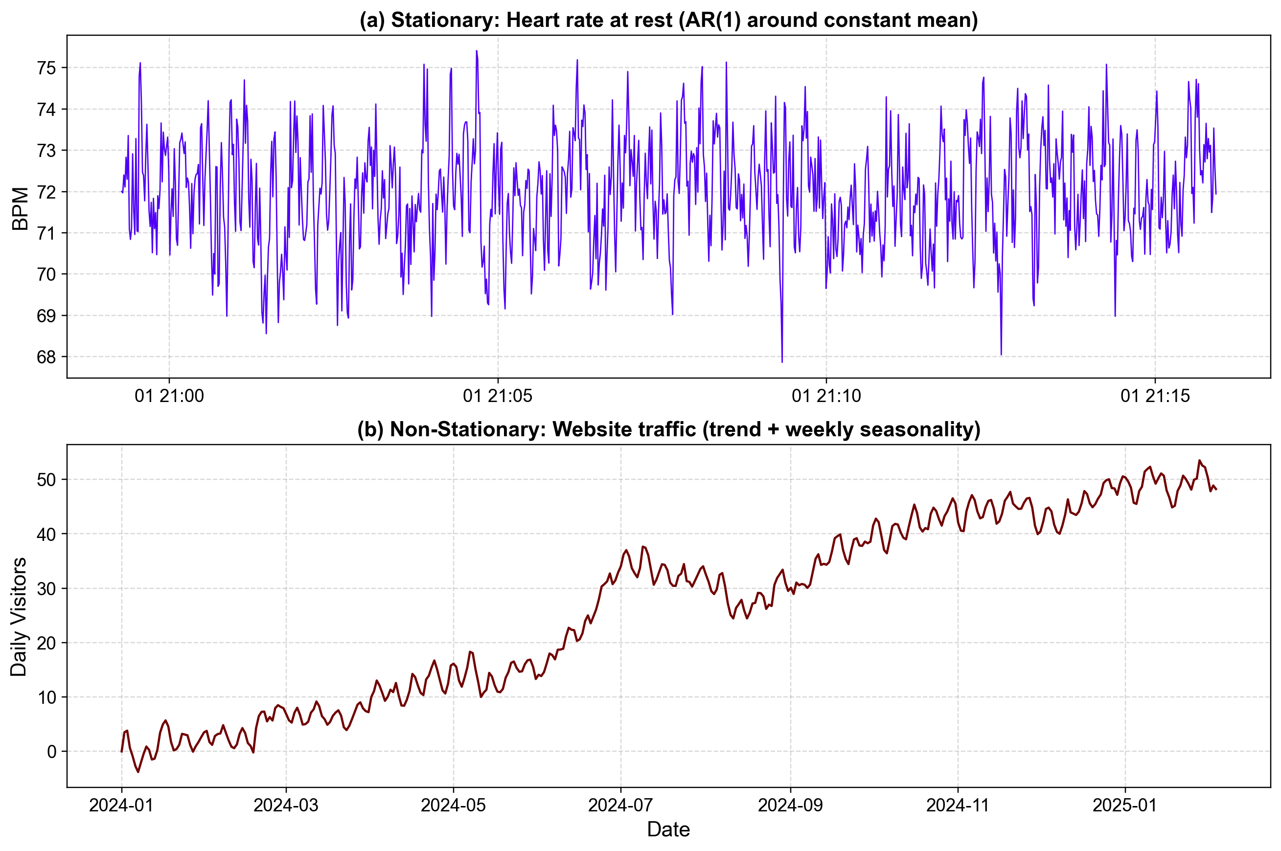
Fig. 3.26 Comparison of Stationary vs. Non-Stationary Processes#
Fig. 3.26 contrasts these two distinct behaviors using our real-world examples:
Top Panel (Stationary Heart Rate): We can see the data “vibrating” around a constant center (our resting heart rate). Notice how the series never escapes its baseline; even when a random spike occurs, it is immediately pulled back toward the middle. Because the average and the spread of the wiggles stay the same throughout the entire timeline, we call this stationary. If we looked at any small slice of this graph, it would look statistically identical to any other slice.
Bottom Panel (Non-Stationary Website Traffic): In our traffic data, the “rules” are constantly shifting. We see a clear upward drift—the mean is higher at the end of the chart than at the beginning. We also see a repeating weekly “wave” (seasonality) that gives the data a specific structure depending on the day of the week. Because the average value and the patterns change as time passes, we call this non-stationary.
Decoding the Jargon: What is an AR(p) Process?
When we look at time series models, we’ll often see terms like AR(1), AR(2), or AR(p). We shouldn’t let the notation scare us—it’s just our way of counting “memory.”
“Autoregressive” (AR) simply means the data predicts itself (auto = self, regressive = prediction).
The number we put in the parentheses tells us how many steps back the memory goes:
AR(1) = “Short-Term Memory”
(3.16)#\[\begin{equation} X_t = \phi X_{t-1} + \epsilon_t \end{equation}\]Our Rule: Today’s value depends only on what happened one step ago (plus some random noise \(\epsilon_t\)).
The Vibe (Heart Rate): We can think of this like a rubber band or a pendulum swinging back to center. In our heart rate example, if the previous second was high, the next one likely stays near it, but the “pull” of the \(\phi\) coefficient ensures the connection fades fast and we return to our average.
AR(2) = “Richer Memory”
(3.17)#\[\begin{equation} X_t = \phi_1 X_{t-1} + \phi_2 X_{t-2} + \epsilon_t \end{equation}\]Our Rule: Today’s value depends on both Yesterday and the Day Before.
The Vibe: This gives our data more complex movements, like a wave that oscillates or bounces. We are remembering not just where we are, but the direction we were coming from.
AR(p) = “Deep Memory”
(3.18)#\[\begin{equation} X_t = \phi_1 X_{t-1} + \phi_2 X_{t-2} + \cdots + \phi_p X_{t-p} + \epsilon_t \end{equation}\]Our Rule: Today depends on the last \(p\) steps.
The Vibe: The higher we set \(p\), the more complex the historical patterns we can capture in our models.
Contrast with our Random Walk (Non-Stationary):
Notice that we have no coefficient pulling us back (unlike the \(\phi\) in our AR model).
Our value just drifts forever based on wherever it was yesterday plus a trend \(\mu\).
In our website traffic example: This is why we see the data “wandering” upward—it lacks the “memory” that pulls it back to a constant mean.
3.5.3. Types of Stationarity#
In time-series analysis, we generally talk about two levels of stationarity: the “impossible ideal” (Strict) and the “practical compromise” (Weak).
Strict Stationarity (The Ideal)
Weak Stationarity (The Practical Standard)
3.5.4. Strict Stationarity#
Strict stationarity [Grenander and Rosenblatt, 2008] represents a very high bar to clear in time series analysis. It demands that the entire probability distribution of your data remains identical, regardless of where you look in time.
In formal terms, for any set of time points and any time shift (or lag) , the joint distributions must be equal:
Practically, this means much more than simply keeping a stable average. It requires every single statistical property—the mean, variance, skewness, kurtosis, and even higher-order moments—to remain frozen in time. If you were to take a snippet of data from January and compare it to another from June, they must be statistically indistinguishable. Furthermore, any relationship you observe today must hold exactly true tomorrow, next week, and in the next century.
To understand this intuitively, consider the example of flipping a fair coin every day for a year. On January 1st, the probability of obtaining Heads is 50%; on December 31st, that probability remains exactly 50%. Even the chance of flipping three Heads in a row remains the same in winter as it does in summer. Because the underlying rules (the physics of the coin) never change and the flips are independent and identical (IID), this process is strictly stationary.
However, applying this in the real world is challenging. While strict stationarity is theoretically useful, it is practically impossible to verify because proving that every possible statistical moment is constant would require infinite data.
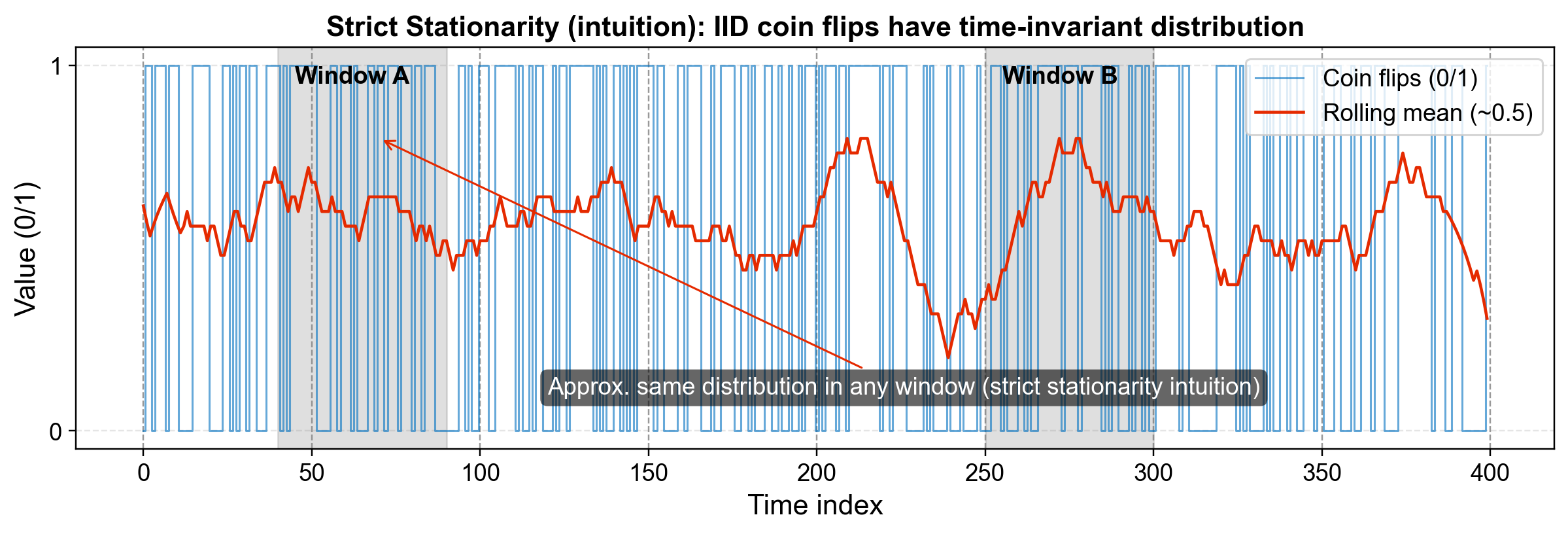
Fig. 3.27 Strict Stationarity: Whether you look at Window A or Window B, the probability distribution (the randomness of the coin) is identical.#
3.5.4.1. Weak Stationarity#
Because strict stationarity [Grenander and Rosenblatt, 2008] is so practically difficult to prove, analysts usually settle for Weak Stationarity (often called Covariance Stationarity). This is the version actually tested for in most econometric models.
In this framework, the requirements are relaxed. We stop worrying about the entire distribution and focus only on the first two “moments.” To achieve weak stationarity, the data must satisfy three specific conditions:
Constant Mean: The average value (\(E[X_t]\)) doesn’t change over time.
Constant Variance: The spread of the data (\(Var(X_t)\)) is stable.
Constant Autocovariance: The relationship between two points depends only on the time distance (lag) between them, not when they occurred.
To see this in action, we often look at an AR(1) process. This type of process is considered weakly stationary because it fluctuates around 0 with a stable variance, and its “memory” fades consistently over time.
To verify this behavior, we use the ACF (Autocorrelation Function). This is our primary tool for visualizing that “memory,” allowing us to confirm that correlations diminish as the time lag increases.
Weak stationary series:
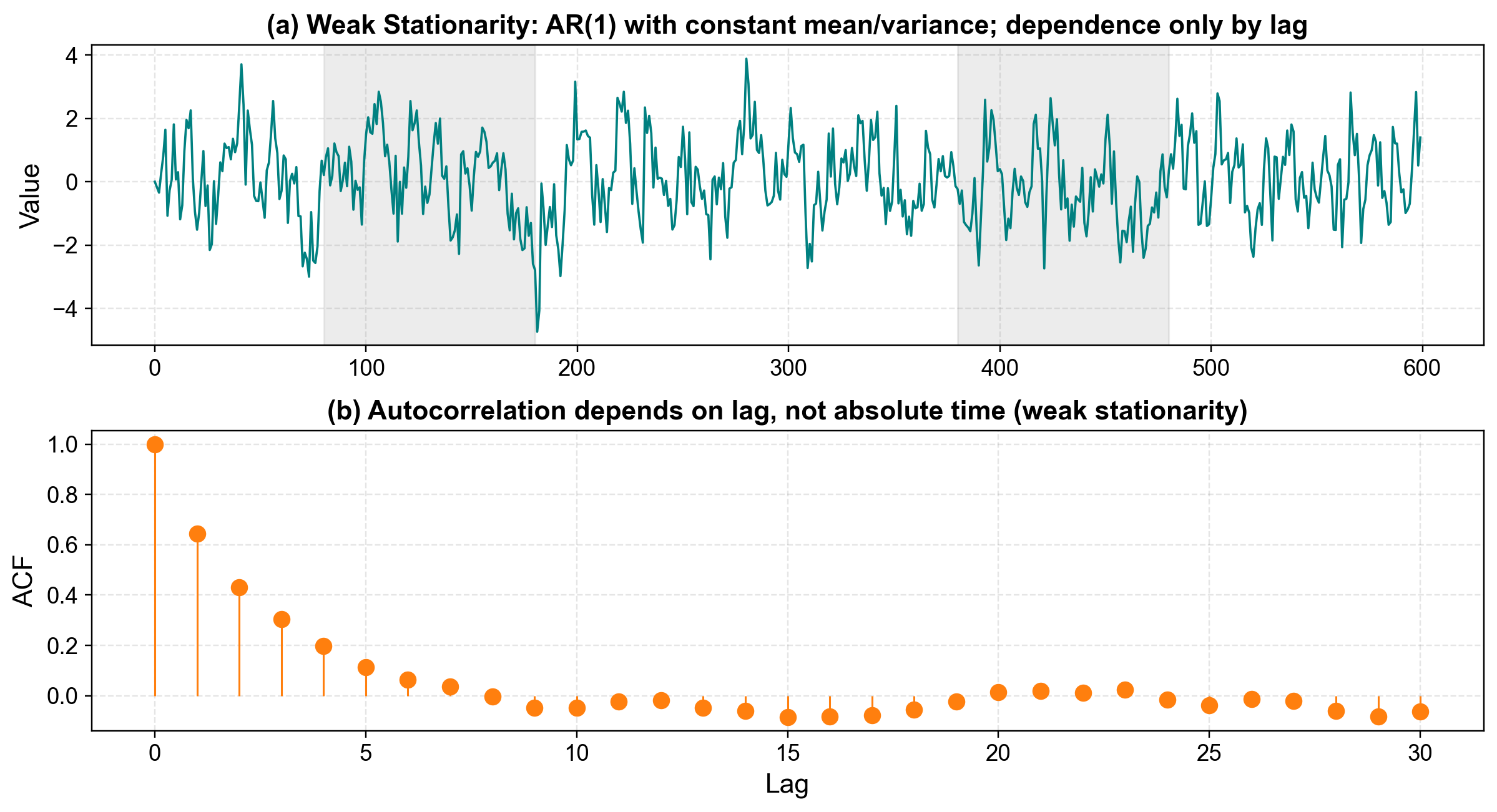
Fig. 3.28 Weak Stationarity: The top panel shows the series fluctuating around a constant mean. The bottom panel (ACF) shows how the “memory” of the process depends only on the time lag.#
3.5.5. The Three Pillars of Weak Stationarity#
To understand weak stationarity [Grenander and Rosenblatt, 2008] fully, we must break down its three essential pillars. Each addresses a different aspect of behavioral stability, starting with the most fundamental: the mean.
3.5.5.1. Condition 1: Constant Mean — The “Center” Never Drifts#
The first condition requires a Constant Mean, meaning the “center” of the data never drifts. Mathematically, this is expressed as:
In practice, this ensures that the long-run average is stable. Whether you examine the first 100 observations or the last, the center of the distribution stays put.
Consider a real-world example of a factory producing widgets. On average, the factory might make 1000 widgets per day. While production naturally fluctuates—hitting 950 on one day and 1050 on another—the average across January, June, and December remains anchored at 1000 units. Crucially, there is no slow drift upward or downward over the year. To visualize this, we can simulate daily production data that varies randomly but adheres strictly to this fixed long-term average.
Segment 1 mean: 1000.8
Segment 2 mean: 995.6
Segment 3 mean: 997.8
Overall mean: 998.1
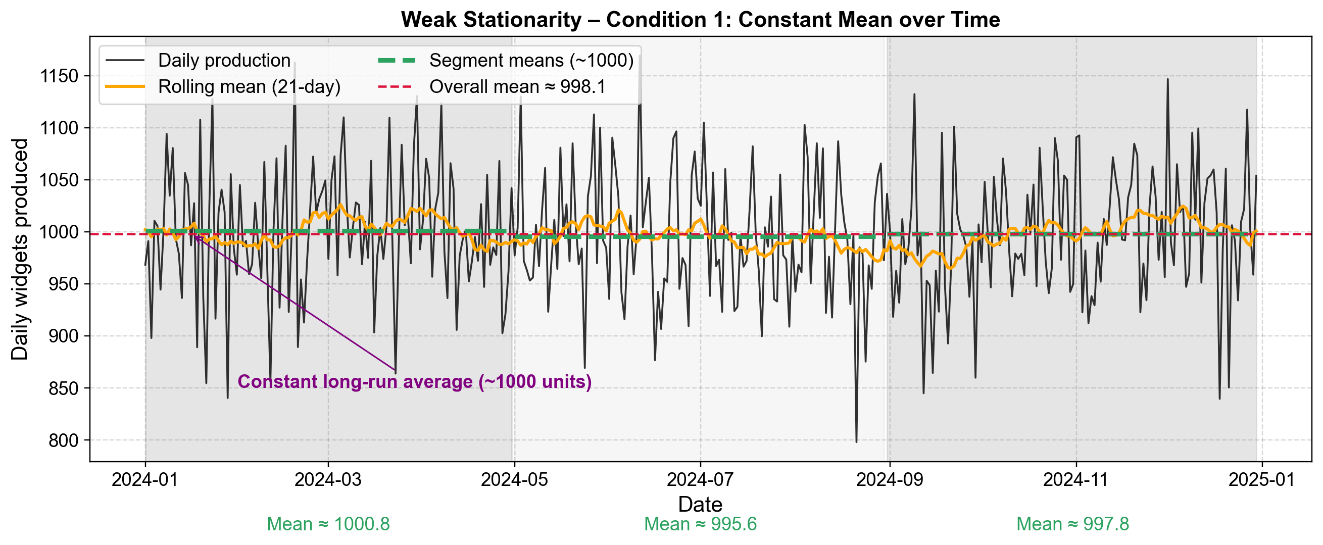
Fig. 3.29 Weak Stationarity – Condition 1: The mean remains constant across the beginning, middle, and end of the series. Notice how the segment means (green dashed lines for three equal segments) all hover around 1000 units.#
3.5.5.2. Condition 2: Finite, Constant Variance — The “Spread” Stays Stable#
Following the requirement for a constant mean, the second condition dictates a Finite, Constant Variance, ensuring the “spread” of the data remains stable. Mathematically, this is defined as [Grenander and Rosenblatt, 2008]:
In practice, this means the amount of variability—or volatility—around the mean does not explode or shrink over time. Good days and bad days happen with roughly the same frequency and magnitude throughout the entire series.
Consider daily stock returns as a real-world example. If the average return is 0.05% per day, and the typical deviation is ±2%, a stationary series maintains this consistency. You do not suddenly see weeks where returns swing wildly by ±10% followed by weeks where they barely move. To illustrate this, we can generate simulated stock returns with stable parameters and visualize how the rolling standard deviation (volatility) stays roughly constant.
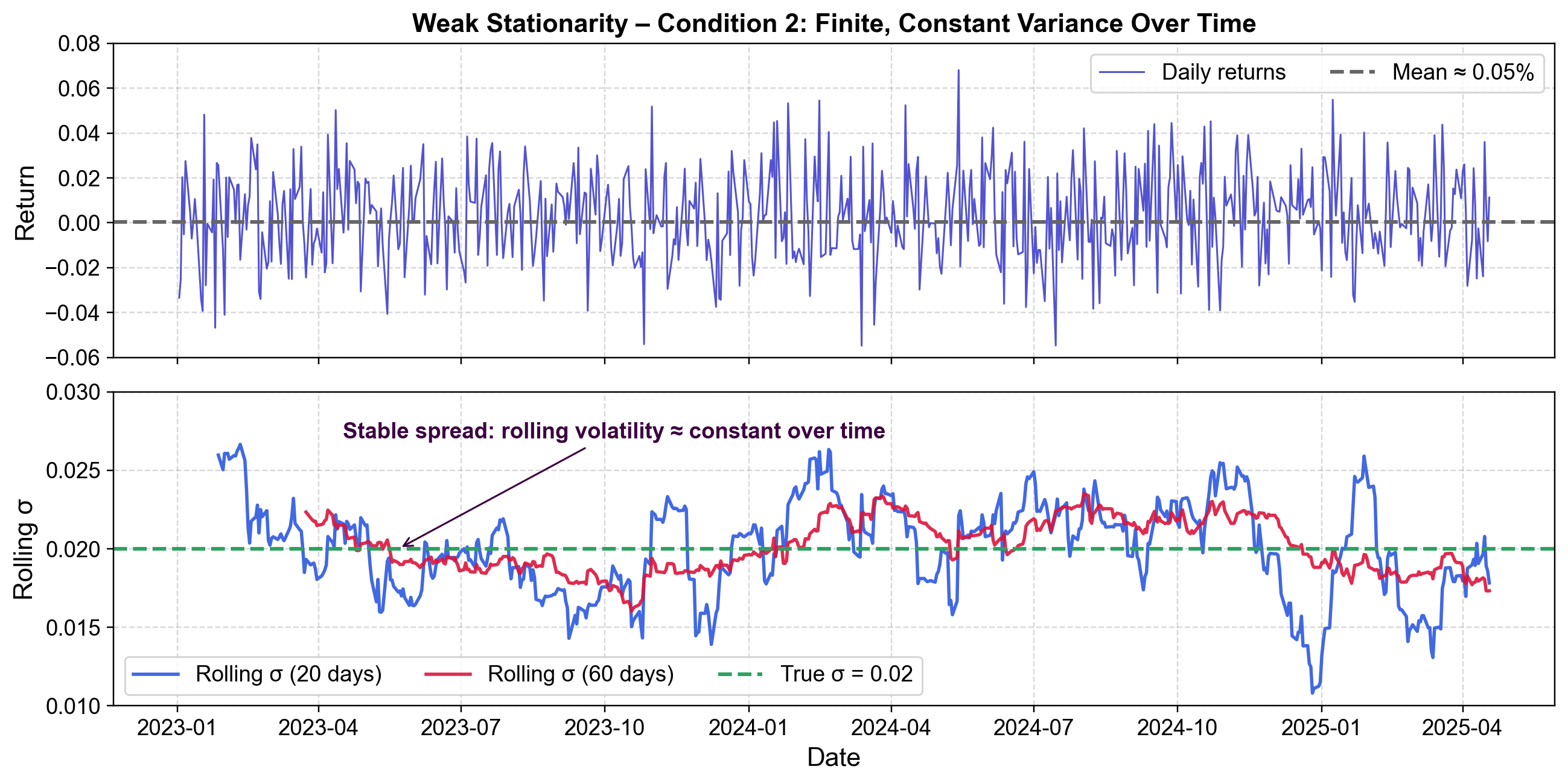
Fig. 3.30 Weak Stationarity – Condition 2: The spread (variance) of the returns stays stable over time. The rolling standard deviation lines hover around the true σ value.#
3.5.5.3. Condition 3: Time-Invariant Covariance — Relationships Depend Only on Distance#
The final piece of the puzzle is Time-Invariant Covariance, which ensures that relationships depend only on distance, not on the calendar date. Mathematically, this condition is expressed as [Grenander and Rosenblatt, 2008]:
n practice, this means the strength of the relationship between observations depends only on how far apart they are in time (\(h\)), not on the specific moment \(t\) when they occurred.
Think about daily temperature as a real-world example. Today’s temperature is usually highly correlated with yesterday’s—perhaps a correlation of 0.8. In a stationary series, this 0.8 correlation holds whether you are observing winter months or summer months. The lag (1 day) determines the relationship, not the season.
A key insight here is that the “memory” of the process is consistent. If you pick two random weeks from your dataset—say, Week 5 and Week 30—and compute the autocorrelation structure within each, they should look nearly identical. To demonstrate this, we can generate a stationary AR(1) process and compare the autocorrelation function (ACF) from two different time windows; if the process is truly stationary, these ACFs will align.
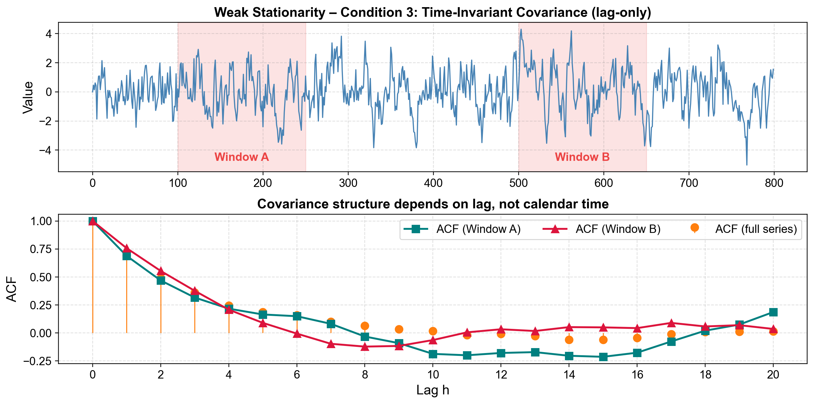
Fig. 3.31 Weak Stationarity – Condition 3: The autocorrelation structure depends only on lag, not calendar time. Window A and Window B are from different periods, yet their ACF curves nearly overlap with the full-series ACF.#
3.5.6. Practical Stationarity Checklist#
When you’re working with real data, you won’t always have the luxury of mathematical proofs. Instead, you need practical heuristics to quickly assess whether your series is behaving in a stationary way. Here are four visual and conceptual checks you can perform.
Good Sign: The data oscillates around the same horizontal level from beginning to end.
Red Flag: You see systematic upward or downward drift over time—the “center” is moving.
Visual Test: Imagine drawing a horizontal line through your data. Does it capture the “average” equally well in January and December?
Good Sign: The “spread” or “width” of fluctuations remains similar across all time periods.
Red Flag: Some periods show wild swings while others are calm (think stock market volatility clustering).
Visual Test: Are the peaks and valleys roughly the same size throughout your dataset?
Good Sign: The pattern of how consecutive observations relate to each other stays consistent over time.
Red Flag: Sometimes observations are highly correlated, other times they appear independent.
Technical Test: The autocorrelation function (ACF) should depend only on the lag \(h\), not on which period you’re analyzing.
⚠️ Be Careful Here
Maybe OK: Regular, repeating patterns can still be stationary (see the special case below).
Red Flag: Seasonal patterns with changing amplitude (e.g., winter variance growing over the years) or shifting timing.
Key Question: Is the seasonal pattern itself evolving over time?
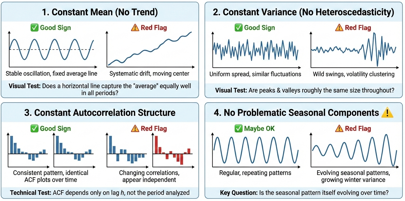
Fig. 3.32 A visual guide to the four key heuristic checks—constant mean, constant variance, consistent autocorrelation, and stable seasonal components—used to assess whether a time series is stationary. (Image generated using Google Gemini).#
3.5.7. Common Stationary Time Series#
Now that we’ve got a feel for what it means for a process to be stationary, let’s take a closer look at two of the most common examples you’ll encounter: white noise and autoregressive (AR) models.
3.5.7.1. White Noise — The “Gold Standard” of Stationarity#
Mathematically, white noise is defined as:
This means that each observation in the series is drawn independently from the same distribution.
Some key features of white noise include:
Independence: Every observation is completely unrelated to the others.
Identical distribution: The underlying probability distribution doesn’t change over time.
Constant mean and variance: \(\mathbb{E}[X_t] = \mu\) and \(\text{Var}[X_t] = \sigma^2\).
Zero autocorrelation: \(\text{Corr}[X_t, X_{t+h}] = 0\) for all \(h \neq 0\).
The most common form of white noise is Gaussian white noise, written as:
You can think of white noise as representing completely random fluctuations without any predictable structure. Examples include measurement errors from a precise instrument, daily stock returns (roughly, under the efficient market hypothesis), regression residuals from a well-fitted model, or even a series of fair coin flips coded as 0 and 1.
White noise matters because it serves as the simplest example of a stationary process and provides a foundation for more complex models. It’s often used as a benchmark—many models can be described as transformations of white noise—and as a diagnostic tool—if your model’s residuals resemble white noise, that’s a sign you’ve captured the underlying patterns of your data well.
Next, we’ll see how white noise extends into something more structured: the autoregressive model.
White Noise Data (first 20 observations):
| white_noise | |
|---|---|
| time | |
| 0 | -1.763172 |
| 1 | -0.574722 |
| 2 | -2.207049 |
| 3 | -2.700853 |
| 4 | 0.195151 |
| 5 | 2.393428 |
| 6 | 1.489741 |
| 7 | -3.545561 |
| 8 | -0.719388 |
| 9 | -2.475573 |
| 10 | -0.815234 |
| 11 | 1.169417 |
| 12 | -0.753913 |
| 13 | 0.428834 |
| 14 | 4.054856 |
| 15 | -0.111775 |
| 16 | -2.055154 |
| 17 | 0.537881 |
| 18 | 0.897075 |
| 19 | -0.460199 |
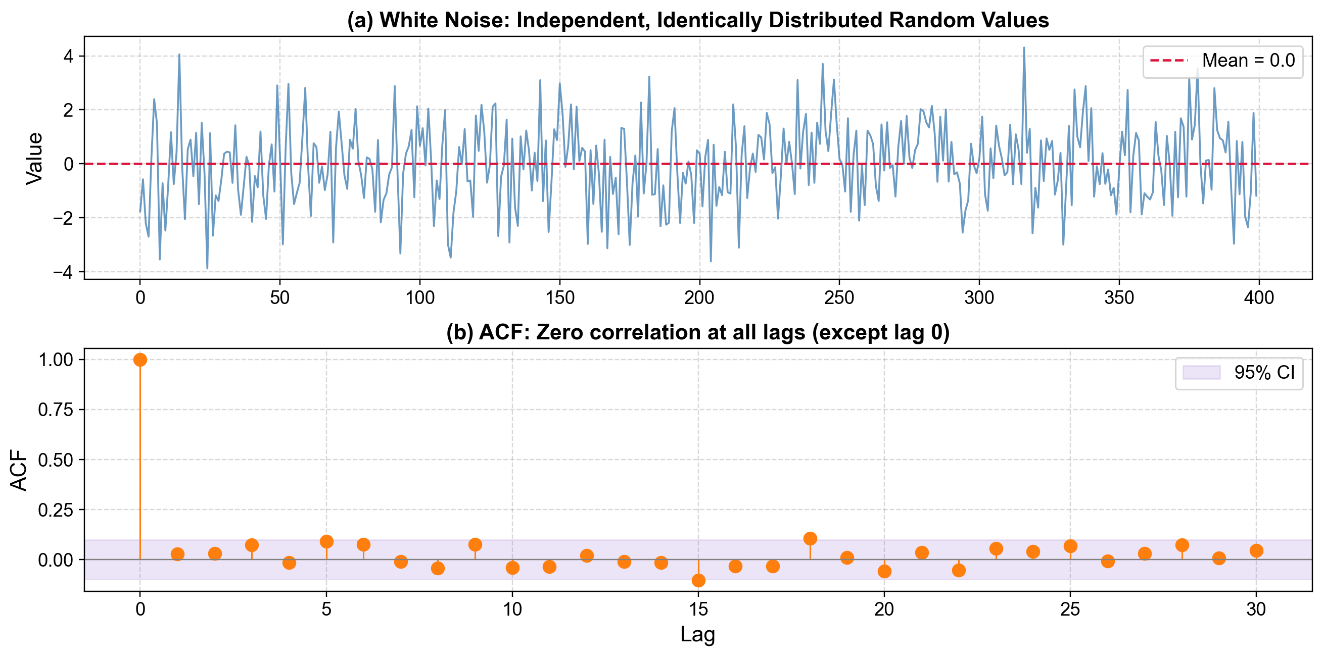
Fig. 3.33 White Noise: The top panel shows completely random, uncorrelated observations. The bottom panel (ACF) shows zero correlation at all lags except lag 0, confirming independence.#
3.5.7.2. Stationary Autoregressive (AR) Processes#
White noise is completely random, but most real-world time series aren’t like that. In reality, what happens today often depends, at least a little, on what happened yesterday. That’s where autoregressive (AR) processes come into play.
The simplest version is the AR(1) model, defined as:
Here, each new value \(X_t\) depends partly on its previous value \(X_{t-1}\) and partly on a random shock \(\epsilon_t\).
Some key characteristics of an AR(1) process are:
Dependence on the past: The coefficient \(\phi\) controls how strongly each value depends on the previous one.
Mean reversion: When the process drifts away from its long-term average, it gradually moves back toward it.
Finite variance: Unlike a random walk, the variability doesn’t blow up over time.
Autocorrelation decay: The correlation between observations decreases exponentially with lag, following \(\text{Corr}[X_t, X_{t+h}] = \phi^h\).
For the process to be stationary, the absolute value of \(\phi\) must be less than 1. When \(|\phi| < 1\), the series is stable and mean-reverting. If \(\phi = 1\), it behaves like a random walk—non-stationary and unpredictable. And if \(|\phi| > 1\), the process becomes explosive, with values that drift off to infinity.
A simple way to visualize this is with the ball and spring analogy. Imagine a ball attached to a spring:
The spring represents the pull of mean reversion.
The shocks (\(\epsilon_t\)) are random pushes that move the ball off its equilibrium position.
The balance between these pushes and the spring’s pull gives rise to the gentle ups and downs of a stationary process.
If \(\phi\) is near 1, the spring is loose—the ball takes a long time to return. If \(\phi\) is smaller (say, 0.3), the spring is tight—pulling the ball back quickly after each shock.
You can find AR(1)-type behavior in many real situations:
Interest rates, which tend to revert toward central bank targets.
Exchange rates, which drift but are pulled toward purchasing power parity.
Commodity prices, shaped by supply-demand adjustments.
Temperature anomalies, which oscillate around long-term climate averages.
Next, we’ll look at how to simulate an AR(1) process and visualize its dynamics in action.
AR(1) Data (first 20 observations):
| ar1_value | |
|---|---|
| time | |
| 0 | 0.000000 |
| 1 | 0.075552 |
| 2 | -1.077743 |
| 3 | -1.405850 |
| 4 | -1.877211 |
| 5 | -2.588149 |
| 6 | -1.872858 |
| 7 | -1.246487 |
| 8 | -0.462428 |
| 9 | -0.896582 |
| 10 | -1.428941 |
| 11 | 0.311776 |
| 12 | 1.492942 |
| 13 | -0.169298 |
| 14 | 0.195211 |
| 15 | -1.308174 |
| 16 | -1.284683 |
| 17 | -1.668505 |
| 18 | -0.775337 |
| 19 | -0.485442 |
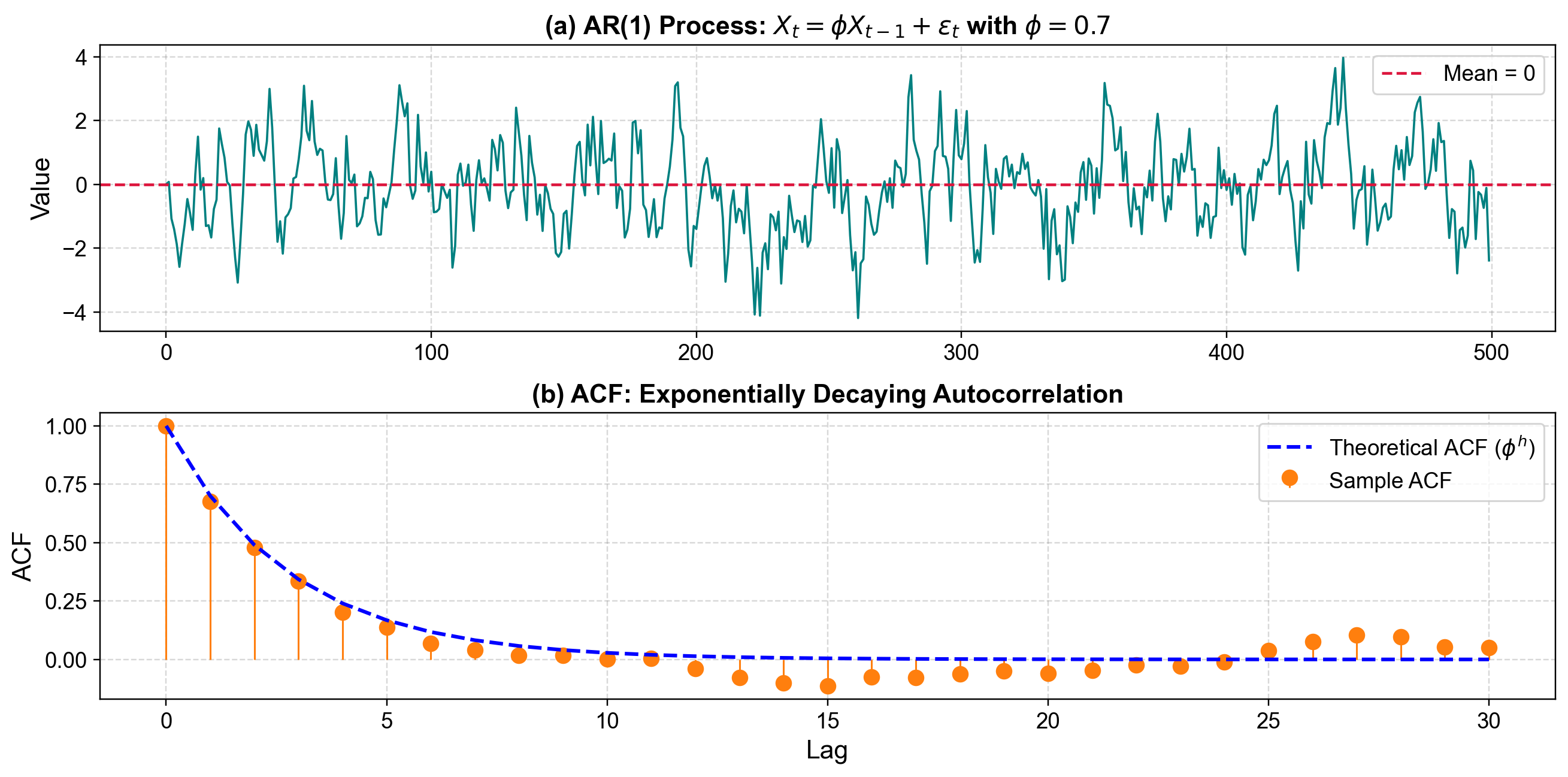
Fig. 3.34 AR(1) Process with φ=0.7: The top panel shows mean-reverting behavior around zero. The bottom panel shows exponentially decaying autocorrelation, with sample ACF (orange) closely matching the theoretical curve (blue dashed line).#
3.5.7.3. Extended AR(p) Process#
So far, we’ve looked at the simplest autoregressive model, where each observation depends only on the previous one. But in many real-world scenarios, today’s value might also be influenced by data from two, three, or even more time steps back. To capture those longer memory effects, we extend the model to an AR(p) process.
The general form looks like this:
Here, \(p\) represents the number of past terms (or “lags”) that help determine the current value \(X_t\).
For the process to be stationary, all roots of the characteristic polynomial must lie outside the unit circle. This is a generalization of the simpler condition \(|\phi| < 1\) that we used for the AR(1) model.
What does adding more lags actually do?
Adds memory: The model can look further back in time, not just one step.
Creates richer patterns: With multiple coefficients, the series can display oscillations, cycles, or more subtle correlations over time.
Remains mean-reverting: Even with more complexity, the process still gravitates back toward its long-term mean.
This added flexibility makes AR(p) models extremely useful in practice. They form the foundation of ARIMA models (the cornerstone of classical time series forecasting) and are widely used in economics, finance, and climate modeling. For instance, GDP growth, unemployment rates, and many macroeconomic indicators often follow AR-like structures.
By adjusting the number of lags and the coefficients, an AR(p) model can fit a wide variety of temporal behaviors—offering a balance between simplicity and the ability to capture real-world dynamics.
Next, we’ll explore how to simulate and visualize an AR(2) process to see how added memory shapes the data’s appearance over time.
AR(2) Data (first 20 observations):
| ar2_value | |
|---|---|
| time | |
| 0 | 0.000000 |
| 1 | 0.000000 |
| 2 | 0.420205 |
| 3 | 0.120762 |
| 4 | 0.962059 |
| 5 | 0.412693 |
| 6 | 1.712811 |
| 7 | -0.567000 |
| 8 | -0.443548 |
| 9 | -0.625700 |
| 10 | 0.936077 |
| 11 | -0.635702 |
| 12 | -0.865037 |
| 13 | 1.196572 |
| 14 | -1.266921 |
| 15 | -0.797223 |
| 16 | 2.514767 |
| 17 | 2.712615 |
| 18 | 2.664726 |
| 19 | 1.591058 |
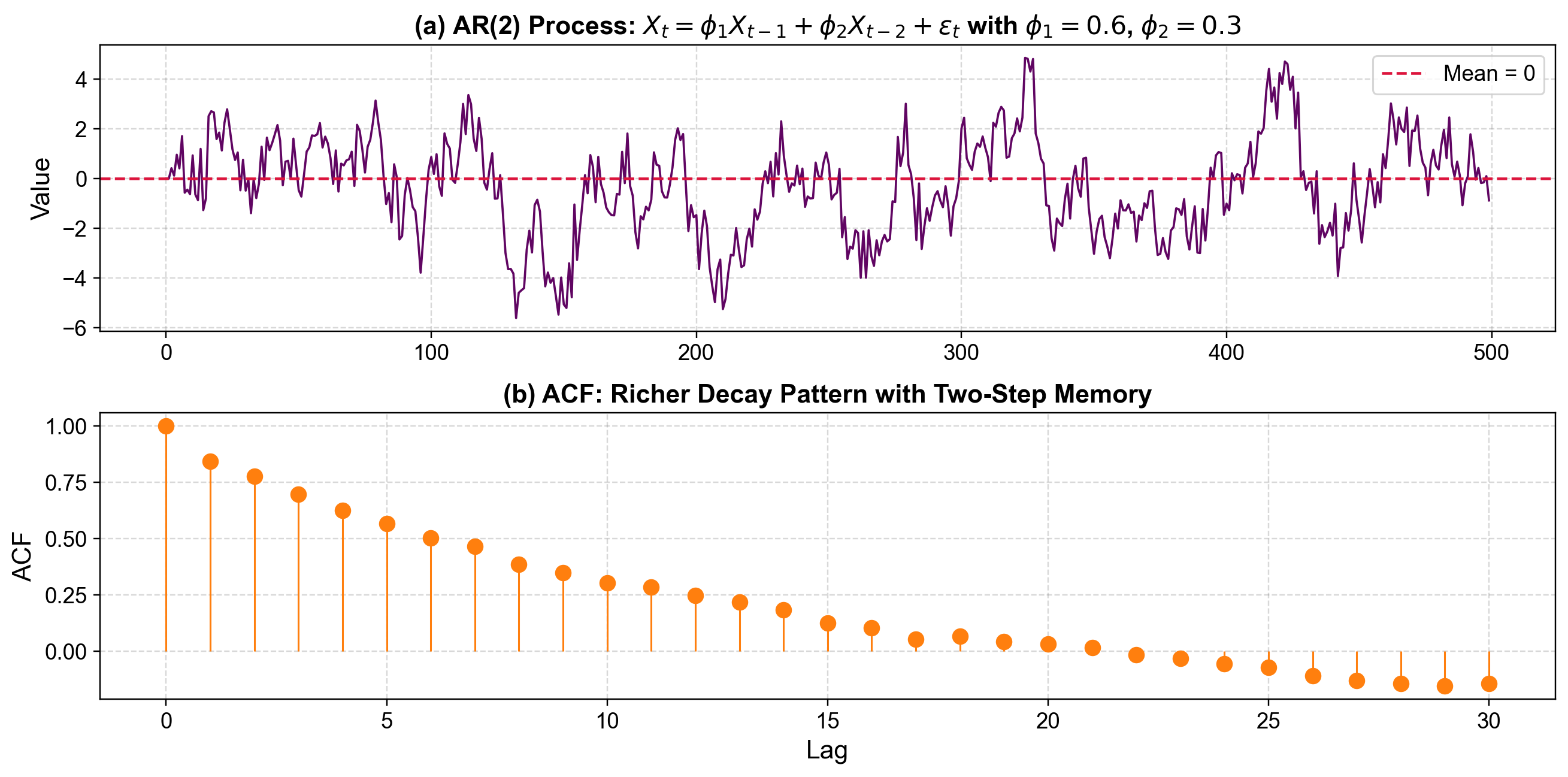
Fig. 3.35 AR(2) Process with φ₁=0.6, φ₂=0.3: The ACF shows a richer decay pattern compared to AR(1), reflecting the influence of two past values rather than one.#
Key Takeaways for This Section
Hierarchy of Stationarity
Strict stationarity → Complete distributional invariance (theoretical ideal, rarely testable).
Weak stationarity → Constant mean, variance, and time-invariant covariance (practical focus).
Practical checklist → Observable characteristics you can spot in real data.
Counter-Intuitive Insights
Periodic ≠ Non-stationary: Regular, repeating patterns can be stationary if their amplitude, frequency, and phase distribution don’t change.
White noise ≠ “No information”: Even purely random data has clear statistical structure (constant mean, variance, zero autocorrelation).
AR processes balance memory and stability: Past dependence doesn’t prevent stationarity as long as the coefficients create mean reversion (\(|\phi| < 1\)).