Remark

Please be aware that these lecture notes are accessible online in an ‘early access’ format. They are actively being developed, and certain sections will be further enriched to provide a comprehensive understanding of the subject matter.

5.1. Outlier Detection in Time Series

5.1.1. Motivation: When One Bad Data Point Ruins Everything

Consider a retailer forecasting demand to optimize inventory. In January 2024, they observe daily sales averaging $15,000. On January 15th, the system records -$12,000—a negative sale. This impossible value stems from a data entry error where a refund was logged incorrectly.

If we naively fit a forecasting model to this contaminated data, the estimated mean drops from $15,000 to $14,672, the variance inflates by 40%, and the trained model persistently under-forecasts February demand by 8%. A single bad value out of 365 observations corrupts the entire pipeline.

This example illustrates why outlier detection is not a cosmetic preprocessing step—it is a fundamental requirement for reliable time series analysis.

5.1.2. What Are Outliers?

Outliers are observations that deviate significantly from the expected pattern established by the majority of the data. In cross-sectional statistics, an outlier might simply be “an unusually large or small value.” In time series, the definition becomes more nuanced: we must ask whether a value is unusual given its temporal context.

5.1.2.1. Time Series Context: Why Location Matters

A daily sales figure of $25,000 could be:

• Normal if it occurs on Black Friday during a holiday promotion

• An outlier if it occurs on a Tuesday in February with no special events

• Suspicious if the previous 30 days averaged $10,000 and there’s no documented reason for the spike

Unlike independent observations, time series outliers depend on:

1. Trend: Is the value unusual relative to the current trajectory?

2. Seasonality: Does it deviate from the expected seasonal pattern?

3. Recent History: Is it inconsistent with the preceding observations?

5.1.2.2. Origins of Outliers

Outliers typically arise from one of three distinct mechanisms, and identifying the source is critical because it dictates your handling strategy:

1. Natural Extremes (Keep Them): These are legitimate, albeit rare, values from the tail of the true distribution—such as record electricity demand during a heatwave or a viral traffic spike. You should retain these because removing them artificially smooths reality, leaving your model unprepared for future extremes that are part of normal business operations.

2. Measurement Errors (Fix or Remove): These are artifacts of data collection failures, such as a broken sensor reporting -999°C, a duplicate transaction, or a typo (e.g., entering $1M instead of $10k). These points contain zero information and purely corrupt your estimates; they must be corrected or deleted to prevent them from biasing your analysis.

3. Exceptional Events (Keep and Flag): These are genuine but non-recurring disturbances caused by external shocks, like a supply chain outage from a hurricane or a cyberattack. While the data is real, treating it as a repeating pattern leads to overfitting. The best approach is to keep the data point but flag it (e.g., with a dummy variable) so the model learns to treat it as a special case rather than a regular occurrence.

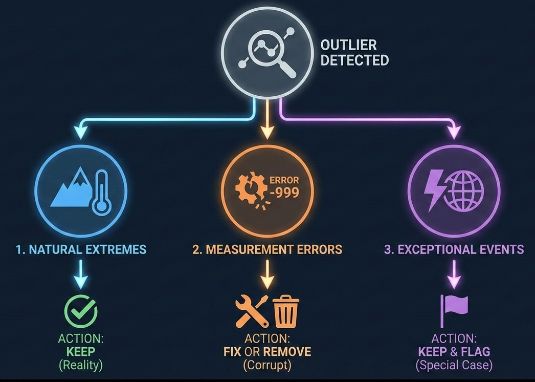
Fig. 5.1 Decision framework for handling outliers. This flowchart summarizes the three critical paths for outlier management. When an outlier is detected, identifying its root cause is the first step. Natural Extremes (e.g., heatwaves) should be kept to preserve reality. Measurement Errors (e.g., sensor failures) are corrupt data points that must be fixed or removed. Exceptional Events (e.g., strikes or disasters) are real but unique; they should be kept in the dataset but flagged (e.g., with a dummy variable) so models treat them as special cases rather than learning them as repeating patterns. (Image generated using Google Gemini).

5.1.3. Why Outlier Detection Matters

5.1.3.1. Impact on Statistical Inference

Outliers exert disproportionate influence on parameter estimates because many statistical methods minimize squared errors. A single extreme value can:

• Bias the Mean: One observation of $100,000 in data averaging $10,000 pulls the mean from $10,000 to $11,944 (assuming 50 observations).

• Inflate Variance: The same outlier increases the standard deviation from $500 to $12,600—a 25-fold increase.

• Distort Correlations: A single spike that coincides with a seasonal peak can create spurious correlation between unrelated variables.

These distortions propagate through every downstream analysis: hypothesis tests lose power, confidence intervals become unreliable, and regression coefficients become biased.

5.1.3.2. Impact on Forecasting Models

Forecasting models learn patterns from historical data. When outliers contaminate training data:

• ARIMA Models: Parameter estimates (AR and MA coefficients) become biased, leading to mis-specified dynamics.

• Exponential Smoothing: The smoothing constant adapts to extreme noise, causing over- or under-reaction to new data.

• Machine Learning: Gradient-based methods (neural networks, gradient boosting) chase outliers during training, sacrificing generalization.

A study of retail demand forecasting found that removing just 2% of observations flagged as outliers reduced Mean Absolute Percentage Error (MAPE) by 15% on average.

5.1.3.3. Dual Nature: Threat and Opportunity

While outliers threaten model validity, they also convey critical information:

• Fraud Detection: Unusual transaction patterns flag potential credit card fraud.

• Equipment Failure: Sensor readings that suddenly spike often precede mechanical failures.

• Market Anomalies: Trading volume outliers may signal insider information or news events.

The goal is not to blindly remove all extreme values, but to detect, investigate, and handle them appropriately based on their origin and business context.

Key Principle

Not all outliers are errors, and not all errors are outliers.

A value can be statistically extreme yet perfectly valid (Black Friday sales), while a subtle data quality issue (systematic 1% under-reporting) may never trigger outlier detection. Effective analysis requires both statistical methods and domain knowledge.

5.1.4. Building a Synthetic E-commerce Dataset

Let’s create a synthetic e-commerce dataset to explore outlier detection. By building it from scratch, we control exactly what patterns exist and, crucially, which values qualify as outliers.

Why Synthetic Data?

In real-world data, the “ground truth” is often unknown—we rarely know for certain whether a spike is a genuine anomaly or just extreme noise. By constructing our own dataset, we can:

1. Define the Baseline: Establish a clear “normal” behavior (trend + seasonality).

2. Control Complexity: Introduce known patterns (like weekend boosts) to see how detection algorithms handle them.

3. Evaluate Accuracy: Precisely measure how well different methods identify the specific anomalies we inject.

5.1.4.1. Step 1: Constructing the Baseline Time Series

We’ll build one year of daily sales data (365 days). Our model will include three fundamental components commonly found in retail data:

1. Trend: A gradual linear increase in sales (simulating business growth).

2. Seasonality: A recurring weekly pattern (simulating higher demand on weekends).

3. Noise: Random day-to-day fluctuations (simulating natural variability).

Mathematical Model

We combine these components using a mixed additive-multiplicative model:

(5.1)\[\begin{equation} \text{Sales}_t = (\text{Trend}_t \times \text{Seasonality}_t) + \text{Noise}_t \end{equation}\]

Where:

• \(\text{Trend}_t = 10,000 + 50t\) (Starts at $10k, grows $50/day)

• \(\text{Seasonality}_t = 1.3\) for weekends, \(1.0\) for weekdays

• \(\text{Noise} \sim \mathcal{N}(0, 500)\)

Implementation:

Show code cell source

Hide code cell source

import pandas as pd
import numpy as np

# Set random seed for reproducibility
np.random.seed(42)

# 1. Generate time index (1 year of daily data)
n_days = 365
dates = pd.date_range('2024-01-01', periods=n_days, freq='D')

# 2. Create base trend component (gradual growth)
base_sales = 10000  # Starting daily sales
growth_rate = 50    # Daily growth
trend = base_sales + growth_rate * np.arange(n_days)

# 3. Add weekly seasonality (weekend boost)
day_of_week = dates.dayofweek  # 0=Monday, 6=Sunday
weekend_mask = (day_of_week >= 5).astype(int)  # 1 for Sat/Sun, 0 otherwise
seasonality = 1.0 + 0.3 * weekend_mask  # 30% boost on weekends

# 4. Add random noise (natural variation)
noise = np.random.normal(0, 500, size=n_days)

# 5. Combine components to create baseline sales
sales_baseline = trend * seasonality + noise

# Create DataFrame
df_baseline = pd.DataFrame({'date': dates, 'sales': sales_baseline})

Before we break the data with outliers, it is critical to understand what “normal” looks like.

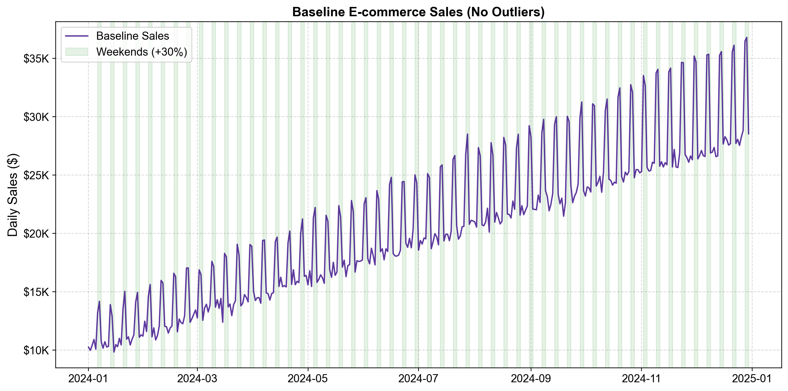
Fig. 5.2 Synthetic E-commerce Sales Baseline (Pre-Outliers). This plot shows the “clean” data generating process before any anomalies are introduced. The purple line tracks daily sales, while green shaded regions indicate weekends. The structure exhibits two key regularities: a deterministic linear trend (sales grow by roughly \(50/day) and clear weekly seasonality (sales spike by 30% every Saturday and Sunday). Notice the "heartbeat" pattern created by these weekend boosts. Crucially, the definition of "normal" evolves over time: a \)15,000 sales day is completely expected in January but would be suspiciously low by December. Any robust outlier detection method must account for this evolving context rather than applying a fixed global threshold [image:38].

Notice the distinct “heartbeat” pattern. The data oscillates regularly due to the weekend boost, and the overall level rises steadily from ~$10k in Jan to ~$30k in Dec. This illustrates why context is king: a raw value of $15,000 is perfectly normal in January but would be a statistically significant anomaly (too low) in December. Effective time series outlier detection requires methods that model this temporal context—comparing each point not to the global average, but to its own local expectation.

5.1.4.2. Step 2: Injecting Realistic Outliers

Now we deliberately add five outliers representing different real-world scenarios. We define them in a dictionary to simulate the specific business context for each anomaly:

Show code cell source

Hide code cell source

outlier_events = {
    85: {'factor': 3.0, 'label': 'Black Friday Sale',
         'reason': 'Major holiday promotion'},
    142: {'factor': 0.6, 'label': 'Website Outage',
          'reason': 'Technical failure'},
    200: {'factor': 2.5, 'label': 'Viral Marketing',
          'reason': 'Social media success'},
    265: {'value': -5000, 'label': 'Data Entry Error',
          'reason': 'Recording mistake'},
    310: {'factor': 2.0, 'label': 'Flash Sale',
          'reason': 'Limited-time promotion'}
}

What Each Outlier Represents

These outliers span the full spectrum of how we should handle extreme values:

• Black Friday (3×): Legitimate extreme event—keep it, this is genuine business activity.

• Website Outage (0.6×): Operational problem—keep but flag for investigation.

• Viral Marketing (2.5×): Unexpected success—keep and analyze what worked.

• Data Entry Error (-$5K): Data quality issue—must correct or remove.

• Flash Sale (2×): Planned promotion—keep it, this reflects real strategy.

Not all outliers deserve the same treatment. Some represent opportunities, others signal problems, and a few are simply mistakes.

We then apply these outliers to our clean baseline series:

Show code cell source

Hide code cell source

# Inject specific outliers with business context
# Apply outliers to a copy of the sales data from the baseline dataframe
sales_contaminated = df_baseline['sales'].copy()

for day_idx, event_info in outlier_events.items():
    if 'factor' in event_info:
        sales_contaminated.iloc[day_idx] = df_baseline['sales'].iloc[day_idx] * event_info['factor']
    elif 'value' in event_info:
        sales_contaminated.iloc[day_idx] = event_info['value']

# Create the final contaminated DataFrame
ecommerce_df = pd.DataFrame({
    'date': dates,
    'sales': sales_contaminated.astype(int),
    'day_of_week': day_of_week,
    'is_weekend': weekend_mask.astype(bool)
})

# Mark outlier dates for easy plotting later
outlier_dates = [dates[idx] for idx in outlier_events.keys()]
ecommerce_df['is_outlier'] = ecommerce_df['date'].isin(outlier_dates)

# Display summary statistics
print("=== Synthetic E-commerce Sales Dataset ===")
print(f"Dataset shape: {ecommerce_df.shape}")
print(f"Date range: {dates[0].date()} to {dates[-1].date()}")
print(f"Number of outliers injected: {len(outlier_events)}")

=== Synthetic E-commerce Sales Dataset ===
Dataset shape: (365, 5)
Date range: 2024-01-01 to 2024-12-30
Number of outliers injected: 5

Now let’s visualize the final dataset with the outliers highlighted. This plot confirms that our synthetic anomalies have been placed correctly and allows us to see how they stand out (or blend in) against the background trend and seasonality.

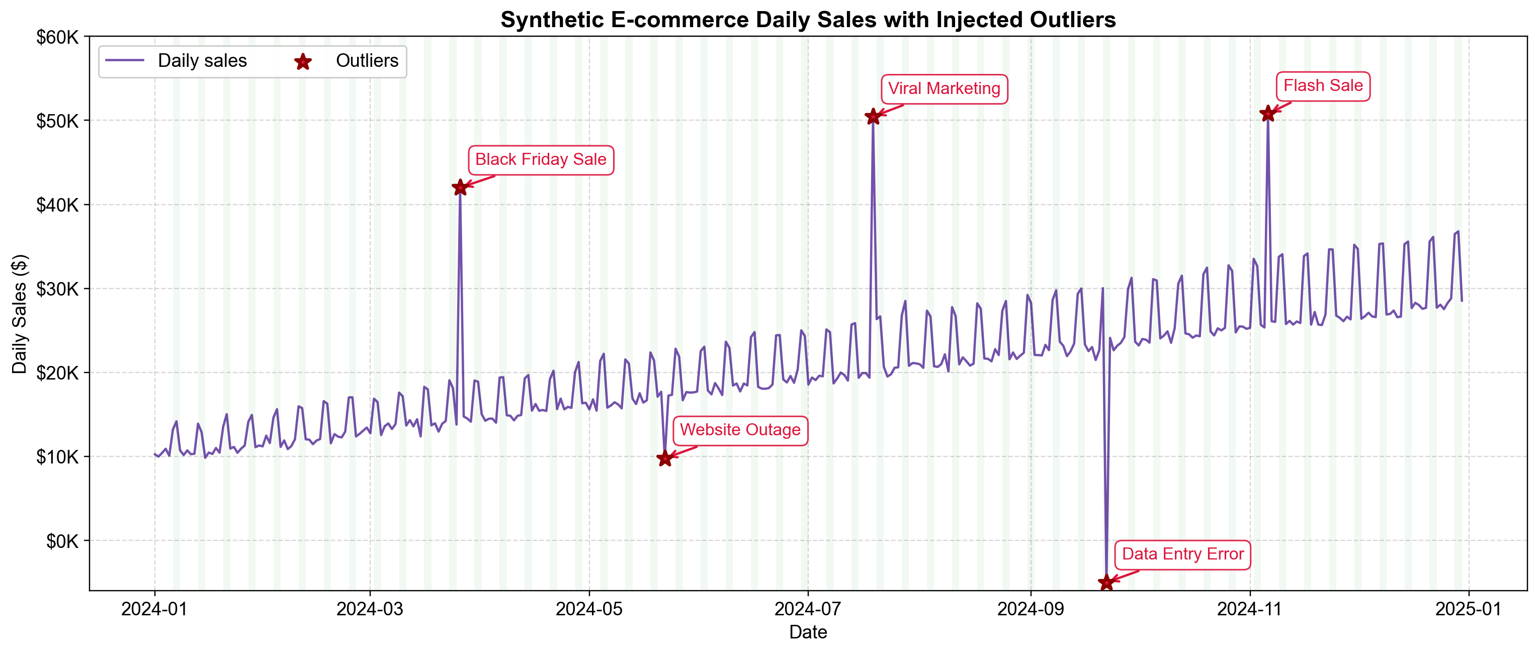
Fig. 5.3 One year of synthetic e-commerce sales with five planted outliers. The series shows steady growth ($50/day), weekly seasonality (weekend boosts highlighted in green), natural day-to-day variation (±$500), and five deliberately injected outliers (red stars). Three spike upward (Black Friday, Viral Marketing, Flash Sale), one drops sharply (Website Outage), and one is physically impossible (Data Entry Error at -$5K). Notice how similar absolute values in March versus November land at different points relative to the baseline—this illustrates why outlier detection must account for temporal context.

Looking at Fig. 5.3, several patterns emerge. The baseline rises steadily throughout the year, creating an upward trend. A regular “sawtooth” pattern repeats every seven days, with weekend periods (shown in green) consistently boosting sales above weekday levels.

The five outliers show distinct behaviors:

1. Black Friday Sale (March): A massive spike to ~$39K, roughly 3x the normal level.

2. Website Outage (May): A sharp drop to ~$8K, reflecting a 40% loss in expected revenue.

3. Viral Marketing (July): An unpredictable surge to ~$40K.

4. Data Entry Error (Sept): A clearly impossible value of -$5,000.

5. Flash Sale (Nov): A doubling of sales to ~$38K.

The Context Problem: Notice that the “Flash Sale” in November (~$38K) is roughly the same absolute dollar value as the “Black Friday” spike in March (~$39K). However, the November value is only 2x its local baseline, while the March value is 3x its local baseline. A simple threshold like “Sales > $35,000” might catch both, but it would fail to distinguish their relative severity given the underlying trend. This reinforces why we need detection methods that respect the time series structure.

5.1.4.3. Step 3: Quantifying the Impact of Outliers

Visualizing data is crucial, but we must also understand how outliers distort our statistical lens. Just five extreme values in a dataset of 365 days (1.4% of the data) can wreak havoc on standard metrics.

The following code generates a comprehensive dashboard comparing the “clean” dataset (if we removed the outliers) against the “contaminated” dataset (what we actually observe).

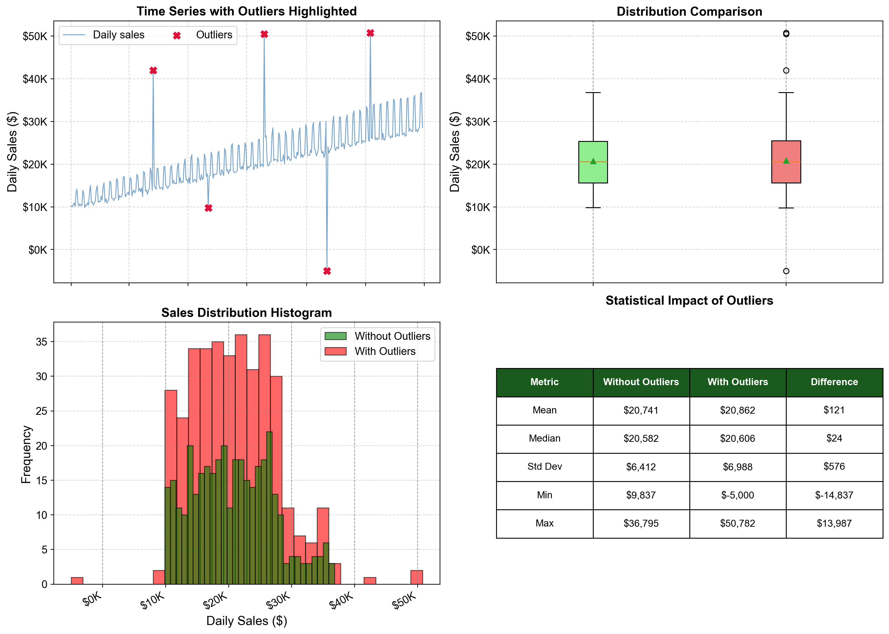
Fig. 5.4 Four perspectives on how outliers affect our data. These visualizations show the same dataset from different angles, revealing how just five outliers (1.4% of observations) influence various statistical measures. The time series (top-left) shows outliers scattered across the year as red X’s. The box plots (top-right) demonstrate how outliers stretch the range from roughly $10K–$37K to -$5K–$50K. Notice the median (central line) barely moves, while the whiskers and outliers expand dramatically. The histogram (bottom-left) reveals “heavy tails”—isolated red bars at -$5K, $40K, and $50K that sit far from the main green distribution. The statistical table (bottom-right) quantifies the damage: while the median remains stable (difference of ~$24), the standard deviation jumps by ~9%, and the range explodes by nearly $30,000.

What This Tells Us

1. Range is Fragile: By doubling the data range (from ~$27k spread to ~$55k spread), outliers destroy the performance of any algorithm that relies on distance or scaling, such as K-Means clustering or Min-Max normalization.

2. Heavy Tails Signal Danger: The isolated bars in the histogram are the visual signature of outliers. They sit far from the main distribution, creating gaps. In forecasting, models (like Neural Networks) often try to “stretch” to cover these gaps, ruining their performance on the normal data.

3. Robustness Matters: Notice how the Median barely budged, while the Mean and Standard Deviation were pulled around. If your outliers are errors (like our -$5k data entry), robust statistics like the Median are your best friends. If they are genuine extremes (like Black Friday), the Mean is telling you the truth about total revenue, but the Median tells you about a “typical day.”