QR factorization

7.5. QR factorization#

Square matrix $A$ can be decomposed as $A = Q R$ where $Q$ is an orthogonal matrix ( $Q^{*} Q = Q Q^{*} = I$ ) and $R$ is an upper triangular matrix. If $A$ is invertible and $R$ is positive, then the factorization is unique.

Furthermore, there are several methods for computing the $Q R$ decomposition such as the Gram–Schmidt process, and the Householder transformations, … Here, we use the Gram–Schmidt process.

Consider matrix $A = [\begin{matrix} | & | & | \\ {\vec{a}}_{1} & {\vec{a}}_{2} & \dots & {\vec{a}}_{n} \\ | & | & | \end{matrix}]$ were ${\vec{a}}_{i}$ are the columns of the full column rank matrix $A$ . Now, define the projection as follows:

\begin{array}{r} {proj}_{\vec{u}} \vec{a} = \frac{⟨ \vec{u}, \vec{a} ⟩}{⟨ \vec{u}, \vec{u} ⟩} \vec{u} \end{array}

Therefore,

\begin{aligned} {\vec{u}}_{1} & = {\vec{a}}_{1}, & {\vec{e}}_{1} & = \frac{{\vec{u}}_{1}}{‖ {\vec{u}}_{1} ‖}, \\ {\vec{u}}_{2} & = {\vec{a}}_{2} - {proj}_{{\vec{u}}_{1}} {\vec{a}}_{2}, & {\vec{e}}_{2} & = \frac{{\vec{u}}_{2}}{‖ {\vec{u}}_{2} ‖}, \\ {\vec{u}}_{3} & = {\vec{a}}_{3} - {proj}_{{\vec{u}}_{1}} {\vec{a}}_{3} - {proj}_{{\vec{u}}_{2}} {\vec{a}}_{3}, & {\vec{e}}_{3} & = \frac{{\vec{u}}_{3}}{‖ {\vec{u}}_{3} ‖}, \\ ⋮ & ⋮ \\ {\vec{u}}_{k} & = {\vec{a}}_{k} - \sum_{j = 1}^{k - 1} {proj}_{{\vec{u}}_{j}} {\vec{a}}_{k}, & {\vec{e}}_{k} & = \frac{{\vec{u}}_{k}}{‖ {\vec{u}}_{k} ‖} . \end{aligned}

Now, ${\vec{a}}_{i}$ can be expressed as

\begin{array}{r} {\begin{cases} {\vec{a}}_{1} = ⟨ {\vec{e}}_{1}, {\vec{a}}_{1} ⟩ {\vec{e}}_{1} \\ {\vec{a}}_{2} = ⟨ {\vec{e}}_{1}, {\vec{a}}_{2} ⟩ {\vec{e}}_{1} + ⟨ {\vec{e}}_{2}, {\vec{a}}_{2} ⟩ {\vec{e}}_{2} \\ {\vec{a}}_{3} = ⟨ {\vec{e}}_{1}, {\vec{a}}_{3} ⟩ {\vec{e}}_{1} + ⟨ {\vec{e}}_{2}, {\vec{a}}_{3} ⟩ {\vec{e}}_{2} + ⟨ {\vec{e}}_{3}, {\vec{a}}_{3} ⟩ {\vec{e}}_{3} \\ ⋮ \\ {\vec{a}}_{k} = \sum_{j = 1}^{k} ⟨ {\vec{e}}_{j}, {\vec{a}}_{k} ⟩ {\vec{e}}_{j} \end{cases} \end{array}

where $⟨ {\vec{e}}_{i}, {\vec{a}}_{i} ⟩ = ‖ {\vec{u}}_{i} ‖$ . This can be written in matrix form:

\begin{aligned} A & = Q R \end{aligned}

\begin{aligned} [\begin{array}{c} a_{11} & a_{12} & \dots & a_{1 n} \\ a_{21} & a_{22} & \dots & a_{2 n} \\ a_{31} & a_{32} & \dots & a_{3 n} \\ ⋮ & ⋮ & ⋮ \\ a_{n 1} & a_{n 2} & \dots & a_{n n} \end{array}] & = [\begin{array}{c} | & | & | \\ {\vec{e}}_{1} & {\vec{e}}_{2} & \dots & {\vec{e}}_{n} \\ | & | & | \end{array}] [\begin{array}{c} ⟨ {\vec{e}}_{1}, {\vec{a}}_{1} ⟩ & ⟨ {\vec{e}}_{1}, {\vec{a}}_{2} ⟩ & ⟨ {\vec{e}}_{1}, {\vec{a}}_{3} ⟩ & \dots & ⟨ {\vec{e}}_{1}, {\vec{a}}_{n} ⟩ \\ 0 & ⟨ {\vec{e}}_{2}, {\vec{a}}_{2} ⟩ & ⟨ {\vec{e}}_{2}, {\vec{a}}_{3} ⟩ & \dots & ⟨ {\vec{e}}_{2}, {\vec{a}}_{n} ⟩ \\ 0 & 0 & ⟨ {\vec{e}}_{3}, {\vec{a}}_{3} ⟩ & \dots & ⟨ {\vec{e}}_{3}, {\vec{a}}_{n} ⟩ \\ ⋮ & ⋮ & ⋮ & ⋱ & ⋮ \\ 0 & 0 & \dots & \dots & ⟨ {\vec{e}}_{n}, {\vec{a}}_{n} ⟩ \end{array}] . \end{aligned}

See [Allaire, Kaber, Trabelsi, and Allaire, 2008, Khoury and Harder, 2016] for the full derivation of this algorithm.

Python Code

import numpy as np
import pandas as pd

def myQR(A):
    '''
    Square matrix $A$ can be decomposed as A=QR
    where Q is an orthogonal matrix and
    R is an upper triangular matrix.

    Parameters
    ----------
    A : numpy array
        DESCRIPTION. Matrix A

    Returns
    -------
    Q : numpy array
        DESCRIPTION. Matrix Q from A = QR
    R : numpy array
        DESCRIPTION. Matrix R from A = QR

    '''
    n = A.shape[0]
    Q = np.zeros([n,n], dtype = float)
    R = np.zeros([n,n], dtype = float)
    A = A.astype(float)
    for j in range(n):
        T = A[:, j]
        for i in range(j):
            R[i, j] = np.dot(Q[:, i], A[:, j])
            T -= R[i, j] * Q[:, i]
        R[j, j] = np.sqrt(np.dot(T, T))
        Q[:, j] = T /R[j, j]
        del T
    return Q, R

MATLAB Code

function [Q, R] = myQR(A)
%{
Square matrix $A$ can be decomposed as A=QR
where Q is an orthogonal matrix and
R is an upper triangular matrix.

Parameters
----------
A : numpy array
    DESCRIPTION. Matrix A

Returns
-------
Q : numpy array
    DESCRIPTION. Matrix Q from A = QR
R : numpy array
    DESCRIPTION. Matrix R from A = QR

%}
n=length(A);
Q =zeros(n,n);
R = zeros(n,n);
for j=1:n
    T = A(:, j);
    for i=1:j
        R(i, j) = dot(Q(:, i), A(:, j));
        T = T - R(i, j) * Q(:, i);
    end
    R(j, j) = sqrt(dot(T, T));
    Q(:, j) = T /R(j, j);
end

import sys
sys.path.insert(0,'..')
import hd_tools as hd

BokehJS 3.1.1 successfully loaded.

Example: Apply QR decomposition on the following matrix and identify $Q$ and $R$ .

\begin{array}{r} A = [\begin{array}{cccc} 7 & 3 & - 1 & 2 \\ 3 & 8 & 1 & - 4 \\ - 1 & 1 & 4 & - 1 \\ 2 & - 4 & - 1 & 6 \end{array}] . \end{array}

Solution: We have,

import numpy as np
from hd_Matrix_Decomposition import myQR
from IPython.display import display, Latex
from sympy import init_session, init_printing, Matrix
A = np.array([ [7, 3, -1, 2], [3, 8, 1, -4], [-1, 1, 4, -1], [2, -4, -1, 6] ])
Q, R = myQR(A)
display(Latex(r'Q ='), Matrix(np.round(Q, 2)))
display(Latex(r'R ='), Matrix(np.round(R, 2)))
display(Latex(r'QR ='), Matrix(np.round(Q@R, 2)))
display(Latex(r'QQ^T ='), Matrix(np.round(Q@(Q.T), 2)))
display(Latex(r'Q^TQ ='), Matrix(np.round((Q.T)@Q, 2)))

Q =

\begin{array}{r} [\begin{array}{c} 0.88 & - 0.12 & 0.11 & - 0.44 \\ 0.38 & 0.75 & - 0.06 & 0.53 \\ - 0.13 & 0.19 & 0.97 & - 0.06 \\ 0.25 & - 0.62 & 0.2 & 0.72 \end{array}] \end{array}

R =

\begin{array}{r} [\begin{array}{c} 7.94 & 4.54 & - 1.26 & 1.89 \\ 0 & 8.33 & 2.25 & - 7.15 \\ 0 & 0 & 3.52 & 0.69 \\ 0 & 0 & 0 & 1.35 \end{array}] \end{array}

Q R =

\begin{array}{r} [\begin{array}{c} 7.0 & 3.0 & - 1.0 & 2.0 \\ 3.0 & 8.0 & 1.0 & - 4.0 \\ - 1.0 & 1.0 & 4.0 & - 1.0 \\ 2.0 & - 4.0 & - 1.0 & 6.0 \end{array}] \end{array}

Q Q^{T} =

\begin{array}{r} [\begin{array}{c} 1.0 & 0 & 0 & 0 \\ 0 & 1.0 & 0 & 0 \\ 0 & 0 & 1.0 & 0 \\ 0 & 0 & 0 & 1.0 \end{array}] \end{array}

Q^{T} Q =

\begin{array}{r} [\begin{array}{c} 1.0 & 0 & 0 & 0 \\ 0 & 1.0 & 0 & 0 \\ 0 & 0 & 1.0 & 0 \\ 0 & 0 & 0 & 1.0 \end{array}] \end{array}

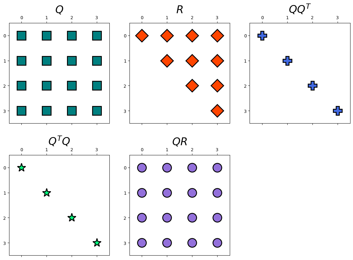
hd.matrix_decomp_fig(mats = [Q, R, np.round(Q@(Q.T), 1), np.round((Q.T)@Q, 1), np.round(np.matmul(Q, R), 2)],
                     labels = ['$Q$', '$R$', '$QQ^T$', '$Q^TQ$', '$QR$'],
                     nrows=2, ncols=3, figsize=(14, 10))

../_images/547fe38696f56261ed0e80f1e71547f8fa9a46bda52dbd6c149cb7acf79727e1.png

Note that we could get a similar results using function, np.linalg.qr.

import scipy.linalg as linalg
Q, R = linalg.qr(A)
display(Latex(r'Q ='), Matrix(np.round(Q, 2)))
display(Latex(r'R ='), Matrix(np.round(R, 2)))
display(Latex(r'QR ='), Matrix(np.round(Q@R, 2)))
display(Latex(r'QQ^T ='), Matrix(np.round(Q@(Q.T), 2)))
display(Latex(r'Q^TQ ='), Matrix(np.round((Q.T)@Q, 2)))

Q =

\begin{array}{r} [\begin{array}{c} - 0.88 & 0.12 & - 0.11 & - 0.44 \\ - 0.38 & - 0.75 & 0.06 & 0.53 \\ 0.13 & - 0.19 & - 0.97 & - 0.06 \\ - 0.25 & 0.62 & - 0.2 & 0.72 \end{array}] \end{array}

R =

\begin{array}{r} [\begin{array}{c} - 7.94 & - 4.54 & 1.26 & - 1.89 \\ 0 & - 8.33 & - 2.25 & 7.15 \\ 0 & 0 & - 3.52 & - 0.69 \\ 0 & 0 & 0 & 1.35 \end{array}] \end{array}

Q R =

\begin{array}{r} [\begin{array}{c} 7.0 & 3.0 & - 1.0 & 2.0 \\ 3.0 & 8.0 & 1.0 & - 4.0 \\ - 1.0 & 1.0 & 4.0 & - 1.0 \\ 2.0 & - 4.0 & - 1.0 & 6.0 \end{array}] \end{array}

Q Q^{T} =

\begin{array}{r} [\begin{array}{c} 1.0 & 0 & 0 & 0 \\ 0 & 1.0 & 0 & 0 \\ 0 & 0 & 1.0 & 0 \\ 0 & 0 & 0 & 1.0 \end{array}] \end{array}

Q^{T} Q =

\begin{array}{r} [\begin{array}{c} 1.0 & 0 & 0 & 0 \\ 0 & 1.0 & 0 & 0 \\ 0 & 0 & 1.0 & 0 \\ 0 & 0 & 0 & 1.0 \end{array}] \end{array}

7.5.1. Solving Linear systems using QR factorization#

We can solve the linear system $A x = b$ for $x$ using QR factorization. To demonstrate this, we use the following example,

Example: Solve the following linear system using QR decomposition.

\begin{array}{r} {\begin{cases} 7 x_{1} + 3 x_{2} - x_{3} + 2 x_{4} = 18 \\ 3 x_{1} + 8 x_{2} + x_{3} - 4 x_{4} = 6 \\ x_{2} - x_{1} + 4 x_{3} - x_{4} = 9 \\ 2 x_{1} - 4 x_{2} - x_{3} + 6 x_{4} = 15 \end{cases} \end{array}

Solution:

Let $A = [\begin{array}{cccc} 7 & 3 & - 1 & 2 \\ 3 & 8 & 1 & - 4 \\ - 1 & 1 & 4 & - 1 \\ 2 & - 4 & - 1 & 6 \end{array}]$ and $b = [\begin{matrix} 18 \\ 6 \\ 9 \\ 15 \end{matrix}]$ . Then, this linear system can be also expressed as follows,

\begin{array}{r} A x = (Q R) x = Q (R x) = b . \end{array}

We have,

A = np.array([ [7, 3, -1, 2], [3, 8, 1, -4], [-1, 1, 4, -1], [2, -4, -1, 6] ])
b = np.array([[18],[ 6],[ 9],[15]])
Q, R = myQR(A)
display(Latex(r'Q ='), Matrix(np.round(Q, 2)))
display(Latex(r'R ='), Matrix(np.round(R, 2)))

Q =

\begin{array}{r} [\begin{array}{c} 0.88 & - 0.12 & 0.11 & - 0.44 \\ 0.38 & 0.75 & - 0.06 & 0.53 \\ - 0.13 & 0.19 & 0.97 & - 0.06 \\ 0.25 & - 0.62 & 0.2 & 0.72 \end{array}] \end{array}

R =

\begin{array}{r} [\begin{array}{c} 7.94 & 4.54 & - 1.26 & 1.89 \\ 0 & 8.33 & 2.25 & - 7.15 \\ 0 & 0 & 3.52 & 0.69 \\ 0 & 0 & 0 & 1.35 \end{array}] \end{array}

Now we can solve the following linear systems instead

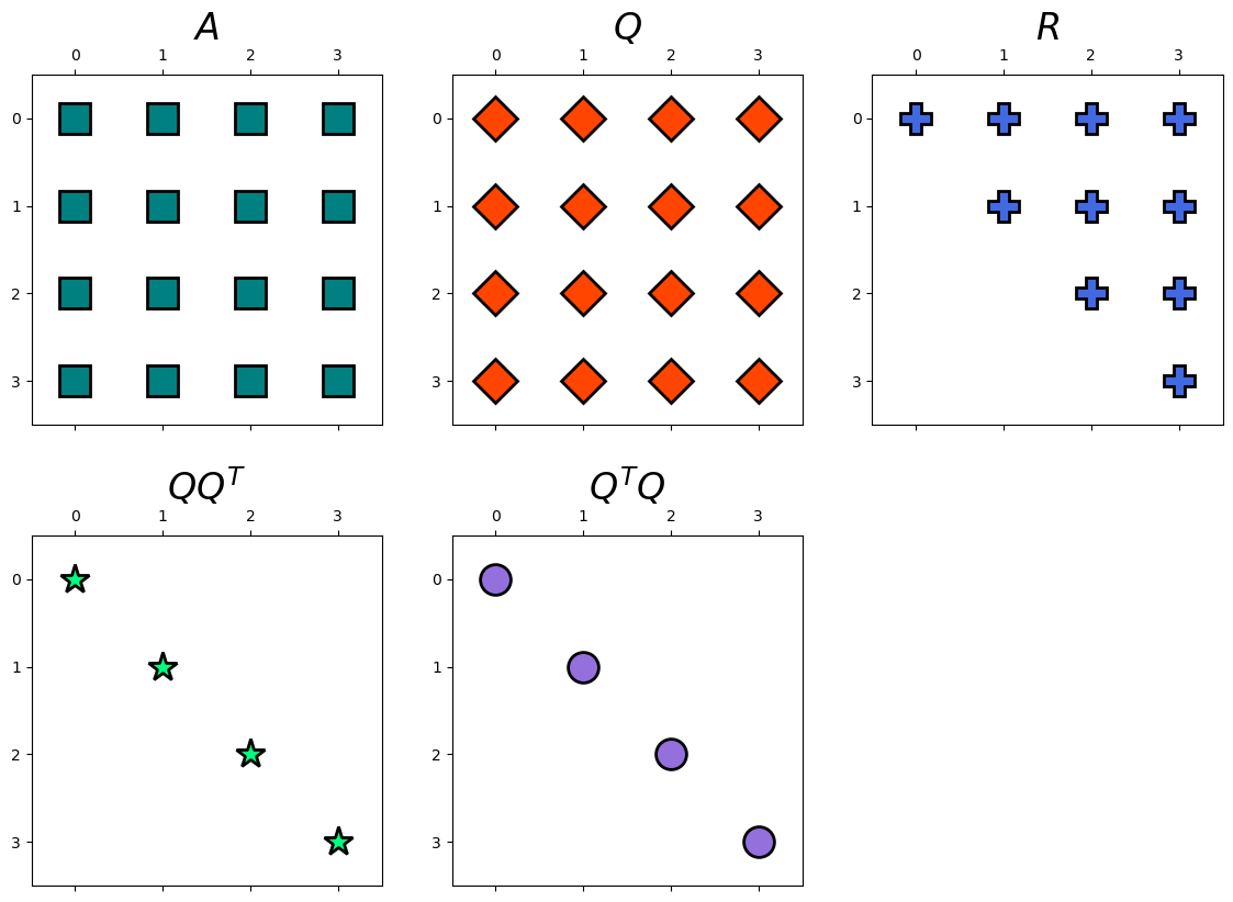
\begin{array}{r} {\begin{cases} Q y = b, \\ R x = y . \end{cases} \end{array}

hd.matrix_decomp_fig(mats = [A, Q, R, np.round(Q@(Q.T), 1), np.round((Q.T)@Q, 1)],
                     labels = ['$A$', '$Q$', '$R$', '$QQ^T$', '$Q^TQ$'],
                     nrows=2, ncols=3, figsize=(14, 10))

../_images/d0a33e4fc92d0b9bc9d42fbb85219714282fe2930a93ab6dd2aed8f440f08094.png

# solving y
y = np.linalg.solve(Q, b)
display(Latex(r'y ='), Matrix(np.round(y, 2)))

y =

\begin{array}{r} [\begin{array}{c} 20.79 \\ - 5.19 \\ 13.32 \\ 5.42 \end{array}] \end{array}

# solving Ux=y for x
x = np.linalg.solve(R, y)
display(Latex(r'x ='), Matrix(np.round(x, 2)))

x =

\begin{array}{r} [\begin{array}{c} 1.0 \\ 2.0 \\ 3.0 \\ 4.0 \end{array}] \end{array}

Let’s now solve the linear system directly and compare the results.

x_new = linalg.solve(A, b)
display(Latex(r'x ='), Matrix(np.round(x_new, 2)))

x =

\begin{array}{r} [\begin{array}{c} 1.0 \\ 2.0 \\ 3.0 \\ 4.0 \end{array}] \end{array}

QR factorization

Contents

7.5. QR factorization#

7.5.1. Solving Linear systems using QR factorization#