3.4. Newton Polynomial

Assume that \(P_{n}(x)\) is the \(n\) degree polynomial such that

(3.37)\[\begin{equation} P_{n}(x) = f(x),\quad x\in\{x_{0},x_{1},x_{2},\ldots,x_{n}\} \end{equation}\]

where \(x_{0}\), \(x_{1}\), \(x_{2}\), \ldots, \(x_{n}\) are distinct points. The \(P_{n}(x)\) can be expressed as follows,

(3.38)\[\begin{equation} P_{n}(x) = a_{0} + a_{1} x^{1} + \ldots + a_{n-1} x^{n-1} + a_{n} x^{n} = \sum_{j = 1}^{n} a_{j} x^{j} \end{equation}\]

or in Lagrange forms from the previous section.

(3.39)\[\begin{equation} L(x)=\sum _{j=0}^{n}y_{j}L_{j}(x) = y_{0} L_{0}(x) + y_{1} L_{1}(x) + \ldots + y_{n} L_{n}(x) \end{equation}\]

Now, there are some challenges when it comes to using the above forms. For example, the coefficients in \(P_{n}(x)\) can be difficult to determine. As for Lagrange, if there is a new data entry the entire process needs to be recalculated. The use of nested multiplication and the relative ease of adding more data points for higher-order interpolating polynomials are advantages of Newton interpolation over Lagrange interpolating polynomials.

Newton polynomial can be also used to interpolate polynomials. This polynomial can be expressed as follows for a sets of distinct data points \(\{ x_{0}, x_{1},\ldots, x_{n}\}\).

(3.40)\[\begin{equation} P_{n}(x) = a_{0} + a_{1} (x - x_{0}) + a_{2} (x - x_{0})(x - x_{1}) + \ldots + a_{n} (x - x_{0})(x - x_{1})\ldots(x - x_{n-1}) \end{equation}\]

where the coefficients \(a_{0}\), \(a_{1}\), \ldots, \(a_{n}\) can be indentured as follows. For example, to find \(a_{0}\),

\[\begin{align*} P_{n}(x_{0}) & = a_{0} + a_{1} (x_{0} - x_{0}) + a_{2} (x_{0} - x_{0})(x_{0} - x_{1}) + \ldots + a_{n} (x_{0} - x_{0})(x_{0} - x_{1})\ldots(x_{0} - x_{n-1})\\ f(x_{0}) & = a_{0} + 0 + 0 + \ldots + 0. \end{align*}\]

Thus,

(3.41)\[\begin{equation} a_{0} = f(x_{0}). \end{equation}\]

Also, for \(a_{1}\), we have,

\[\begin{align*} P_{n}(x_{1}) & = a_{0} + a_{1} (x_{1} - x_{0}) + a_{2} (x_{1} - x_{0})(x_{1} - x_{1}) \\& + \ldots + a_{n} (x_{1} - x_{0})(x_{1} - x_{1})\ldots(x_{1} - x_{n-1}),\\ f(x_{1}) & = a_{0} + a_{1} (x_{1} - x_{0}),\\ \Rightarrow \quad f(x_{1}) & = f(x_{0}) + a_{1} (x_{1} - x_{0}). \end{align*}\]

(3.42)\[\begin{equation} a_{1} = \frac{f(x_{1}) - f(x_{0})}{x_{1} - x_{0}} \end{equation}\]

The 0th Divided Difference of the function \(f\) with respect to \(x_{k}\) is defined as follows,

(3.43)\[\begin{equation} f[x_{k }] =y_{k },\qquad k \in \{0,\ldots ,n\}. \end{equation}\]

Similarly, the 1st Divided Difference of the function \(f\) with respect to \(x_{k}\) and \(x_{k+1}\) is defined as follows,

(3.44)\[\begin{equation} f[x_{k },~x_{k +1}]= \frac {y_{k+1 } - y_{k }}{x_{{k +1}}-x_{k }},\qquad k \in \{0,\ldots ,n-1\}. \end{equation}\]

The 2nd Divided Difference of the function \(f\) with respect to \(x_{k}\), \(x_{k+1}\) and \(x_{k+2}\) is defined as follows,

(3.45)\[\begin{equation} f[x_{k },~x_{k +1},~x_{k +2}]= \frac {f[x_{k+1 },~x_{k +2}] - f[x_{k },x_{k +1}]}{x_{{k +2}}-x_{k }},\qquad k \in \{0,\ldots ,n-2\}. \end{equation}\]

The 3rd Divided Difference:

(3.46)\[\begin{equation} f[x_{k },~x_{k +1},~x_{k +2},~x_{k +3}]= \frac {f[x_{k+1 },~x_{k +2},~x_{k +3}] - f[x_{k },~x_{k +1},~x_{k +2}]}{x_{{k +3}}-x_{k }},\qquad k \in \{0,\ldots ,n-3\}. \end{equation}\]

The jth Divided Difference:

(3.47)\[\begin{equation} f[x_{k },\ldots ,~x_{k +j}]={\frac {f[x_{{k +1}},\ldots ,~x_{{k +j}}]-f[x_{{k }},\ldots ,~x_{{k +j-1}}]}{x_{{k +j}}-x_{k }}},\qquad k \in \{0,\ldots ,n-j\},\ j\in \{1,\ldots ,n\}. \end{equation}\]

The process ends with the single The nth Divided Difference:

(3.48)\[\begin{equation} f[x_{0},~x_{1},\ldots ,~x_{{n}}]=\frac{f[x_{1},~x_{2},\ldots ,~x_{n}]-f[x_{0},~x_{1},\ldots ,~x_{n-1}]}{x_{n}-x_{0}}. \end{equation}\]

(3.49)\[\begin{equation} f[x_{0},~x_{1},\ldots ,~x_{{n}}]=\frac{f[x_{1},~x_{2},\ldots ,~x_{n}]-f[x_{0},~x_{1},\ldots ,~x_{n-1}]}{x_{n}-x_{0}}. \end{equation}\]

Now, let \(a_{0} = f[x_{0}]\) and

(3.50)\[\begin{align} a_{k} &= f[x_{0},~x_{1},\ldots ,~x_{{k}}], \qquad k\in \{1,\ldots ,n\},\\ n_{k}(x)&= \begin{cases} 1, & k = 0,\\ \displaystyle{\prod_{{i=0}}^{{k-1}}(x-x_{i})}, & k>0. \end{cases} \end{align}\]

to be Newton coefficients and Newton basis polynomials, respectively. Then, the Newton interpolation polynomial is a linear combination of Newton basis polynomials

\[\begin{equation*} {P_{n}(x) =\sum _{{k=0}}^{{n}}a_{{k}}n_{{k}}(x) = f[x_{0}] + \sum _{{k=1}}^{{n}} f[x_{0},~x_{1},\ldots ,~x_{{k}}] \prod _{{i=0}}^{{k-1}}(x-x_{i})} \end{equation*}\]

The 1st and 2nd divided differences can be written in the form of a table.

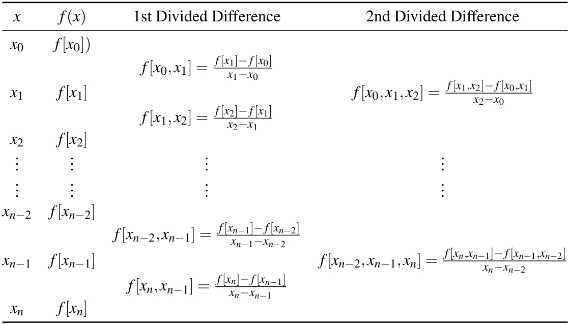
Fig. 3.2 Divided Differences for \(f(x)\)

Python Code

import numpy as np
import pandas as pd

def NewtonCoeff(xn, yn, Frame = False):
    '''
    Parameters
    ----------
    xn : list/array
        DESCRIPTION. a list/array consisting points x0, x1, x2,... ,xn
    yn : list/array
        DESCRIPTION. a list/array consisting points
        y0 = f(x0), y1 = f(x1),... ,yn = f(xn)
    Frame : TYPE, optional
        DESCRIPTION. The default is False.

    Returns
    -------
    TYPE frame or, coefs
        DESCRIPTION.

    '''
    
    n = len(xn)
    #Construct table and load xy pairs in first columns
    A = np.zeros((n,n+1))
    A[:,0]= xn[:]
    A[:,1]= yn[:]
    #Fill in Divided differences
    for j in range(2,n+1):
        for i in range(j-1,n):
            A[i,j] = (A[i,j-1]-A[i-1,j-1]) / (A[i,0]-A[i-j+1,0])
    #Copy diagonal elements into array for returning
    a = np.zeros(n)
    for k in range(0,n):
        a[k] = A[k,k+1]
    if Frame:
        Cols = ['xi','yi']
        temp = 'f[xi'
        for i in range(A.shape[1]-2):
            temp += ', xi+%i'% (i+1)
            Cols.append(temp + ']')
        Table = pd.DataFrame(A, columns=Cols)
        return a, Table
    else:
        return a

def NewtonPoly(x, xn, yn):
    '''
    Parameters
    ----------
    x : TYPE
        DESCRIPTION.
    xn : list/array
        DESCRIPTION. a list/array consisting points x0, x1, x2,... ,xn
    yn : list/array
        DESCRIPTION. a list/array consisting points
        y0 = f(x0), y1 = f(x1),... ,yn = f(xn)

    Returns
    -------
    p : float
        DESCRIPTION. P_n(x)

    '''
    
    n = len(xn)
    # coefficients
    a = NewtonCoeff(xn, yn)
    p = a[n-1]
    for i in range(n-2,-1,-1):
        p = p*(x-xn[i]) + a[i]
    return p

MATLAB Code

function [a] = NewtonCoeff(xn, yn)
%{
Parameters
----------
xn : list/array
    DESCRIPTION. a list/array consisting points x0, x1, x2,... ,xn
yn : list/array
    DESCRIPTION. a list/array consisting points
    y0 = f(x0), y1 = f(x1),... ,yn = f(xn)
Frame : TYPE, optional
    DESCRIPTION. The default is False.

Returns
-------
TYPE a list
    DESCRIPTION. coefs

%}
    
n = length(xn);
% Construct table and load xy pairs in first columns
A = zeros(n,n);
A(:,1)= yn;
% Fill in Divided differences
for i = 2:n
    for j = 2:i
        A(i,j)=(A(i,j-1)-A(i-1,j-1))/(xn(i)-xn(i-j+1));
    end
end
a = diag(A);
end

function p = NewtonPoly(x, xn, yn)
%{
Parameters
----------
x : TYPE
    DESCRIPTION.
xn : list/array
    DESCRIPTION. a list/array consisting points x0, x1, x2,... ,xn
yn : list/array
    DESCRIPTION. a list/array consisting points
    y0 = f(x0), y1 = f(x1),... ,yn = f(xn)

Returns
-------
p : float
    DESCRIPTION. P_n(x)
Example:
xn = [-2, 1 , 3 , 5 , 6, 7];
yn = [-5, -3 ,-1 , 1 , 4, 10]
x = linspace(min(xn)-1 , max(xn)+1 , 100);
%}

n = length(xn);
% coefficients
a = NewtonCoeff(xn, yn);
p = a(n);
for i = n-1:-1:1
    p = p.*(x-xn(i)) + a(i);
end
end

Example: Consider the following data points

\[\begin{align*} \{(1,-3),~(2,0),~(3,-1),~(4,2),~(5,1),~(6,4)\}. \end{align*}\]

Construct an interpolating polynomial using the Newton divided-difference formula and all of this data.

Solution:

# This part is used for producing tables and figures
import sys
sys.path.insert(0,'..')
import hd_tools as hd
import numpy as np
from hd_Interpolation_Algorithms import NewtonPoly, NewtonCoeff

# A set of distinct points
xn = np.array ([-2, 1 , 3 , 5 , 6, 7])
yn = np.array ([-5, -3 ,-1 , 1 , 4, 10])

_, Table = NewtonCoeff(xn, yn, Frame = True)
display(Table.style.set_properties(subset=['xi', 'yi'], **{'background-color': 'black', 'color': 'PaleGreen',
       'border-color': 'DarkGreen'}).format(dict(zip(Table.columns.tolist(),len(Table.columns)*["{:.4f}"]))))
x = np.linspace( xn.min()-1 , xn.max()+1 ,100)
y = NewtonPoly( x , xn , yn )
hd.interpolation_method_plot(xn, yn, x, y, title = 'Newton Method')

Loading BokehJS ...

	xi	yi	f[xi, xi+1]	f[xi, xi+1, xi+2]	f[xi, xi+1, xi+2, xi+3]	f[xi, xi+1, xi+2, xi+3, xi+4]	f[xi, xi+1, xi+2, xi+3, xi+4, xi+5]
0	-2.0000	-5.0000	0.0000	0.0000	0.0000	0.0000	0.0000
1	1.0000	-3.0000	0.6667	0.0000	0.0000	0.0000	0.0000
2	3.0000	-1.0000	1.0000	0.0667	0.0000	0.0000	0.0000
3	5.0000	1.0000	1.0000	0.0000	-0.0095	0.0000	0.0000
4	6.0000	4.0000	3.0000	0.6667	0.1333	0.0179	0.0000
5	7.0000	10.0000	6.0000	1.5000	0.2083	0.0125	-0.0006

Theorem

Assume that \(f \in C^n[a, b]\) and data points \(\{ x_{0}, x_{1},\ldots, x_{n}\}\) from \([a,b]\) are distinct. Then, there is a number \(\xi \in (a, b)\) such that

(3.51)\[\begin{equation} f[x_{0},x_{1},\ldots ,~x_{{n}}] = \frac{f^{(n)} (\xi)}{n!}. \end{equation}\]

Proof:

Define \(g(x) = f(x) - P_{n}(x)\). Now, since \(f(x) = P_{n}(x)\) for all \(x \in \{ x_{0}, x_{1},\ldots, x_{n}\}\), then \(g(x) = 0\) for all \(x \in \{ x_{0}, x_{1},\ldots, x_{n}\}\). Therefore, \(g(x)\) has \(n+1\) unique zeros in \([a,b]\). It follows from Generalized Rolle’s Theorem that there is a number \(\xi \in (a, b)\) such that

(3.52)\[\begin{align} g^{(n)} (\xi) &= 0\\ f^{(n)}(x) - P_{n}^{(n)}(x) &= 0 \end{align}\]

On the other hand, Since \(P_{n}(x)\) is a \(n\) degree polynomial with leading coefficient is \(f[x_{0},x_{1},\ldots ,~x_{{n}}]\). Therefore,

(3.53)\[\begin{equation} P_{n}(x) = n! f[x_{0},x_{1},\ldots ,~x_{{n}}] \end{equation}\]

Thus,

(3.54)\[\begin{equation} f[x_{0},x_{1},\ldots ,~x_{{n}}] = \frac{f^{(n)} (\xi)}{n!} \end{equation}\]

3.4.1. Newton Forward Differences

Recall that forward difference notation \(\Delta\). Given equidistantly distributed data points, we can define Newton forward differences. Note that this is a particular case of Newton polynomials. Given n data points, we have,

\[\begin{align*} \left\{(x_{0},y_{0}),~(x_{1},y_{1}),\ldots ,(x_{n},y_{n}) \right\} \end{align*}\]

where \(y_{j} = f(x_{j})\) for \(0\leq j \leq n\) and

\[\begin{align*} x_{j} = x_{0} + jh,\qquad h>0, ~ 0\leq j \leq n. \end{align*}\]

Note that \(h = \Delta x_{j} = x_{j+1} -x_{j}\). Then, the divided differences can be calculated via forward differences defined as

\[\begin{align*} f[x_{0}] &=y_{0 },\\ f[x_{0 },~x_{1}]&= \frac {f[x_{1}] - f[x_{0}] }{x_{{1}}-x_{0}} = \frac {y_{1 } - y_{0 }}{x_{{1}}-x_{k }} = \frac{\Delta y_{0 }}{h},\\ f[x_{0 },~x_{1},~x_{2}]&= \frac {f[x_{1 },~x_{2}] - f[x_{1 },x_{0}]}{x_{2}-x_{0 }} = \frac {1}{2h}\left(\frac{\Delta y_{1}}{h} - \frac{\Delta y_{0}}{h}\right) = \frac{1}{2!h^2}\Delta^2 y_{0 },\\ &~~ \vdots\\ f[x_{0},\ldots ,~x_{k}]&=\frac{1}{k!h^k}\Delta^k y_{0 },\qquad k\in \{1,\ldots ,n\}. \end{align*}\]

Therefore, the Newton Forward-Difference Formula can be found as follows,

\[\begin{align*} P_{n}(x) = y_{0} + \sum_{k = 1}^{n} \binom{s}{k} \Delta^{k} y_{0}, \end{align*}\]

where \(s = \dfrac{x - x_{0}}{h}\). The above equation can be also expressed as follows,

\[\begin{align*} P_n(x) &= y_{0} + s \Delta^{1} y_{0} + \frac{s(s-1)}{2!} \Delta^{2} y_{0} + \frac{s(s-1)(s-2)}{3!} \Delta^{3} y_{0} \\ &+ \ldots + \frac{s(s-1)(s-2)\ldots(s-n+1)}{n!} \Delta^{n} y_{0}. \end{align*}\]

Python Code

import numpy as np
import pandas as pd
from scipy.special import binom

def ForwardNewton(x, xn, yn, Frame = False):
    '''
    Parameters
    ----------
    x : float
        DESCRIPTION. point x
    xn : list/array
        DESCRIPTION. a list/array consisting points x0, x1, x2,... ,xn
    yn : list/array
        DESCRIPTION. a list/array consisting points
        y0 = f(x0), y1 = f(x1),... ,yn = f(xn)
    Frame : TYPE, optional
        DESCRIPTION. The default is False.

    Returns
    -------
    TYPE frame or, coefs
        DESCRIPTION.

    '''
    h = xn[1]- xn[0]
    n = xn.shape[0]
    A = np.zeros([n,n],dtype = float)
    A[:,0] = yn
    for i in range(1, n):
        A[i:,i] = (A[i:,i-1] - A[i-1:-1,i-1])
    df = np.diag(A)
    # Newton's forward difference formula for variable x
    s = (x - xn[0])/h
    Pn = df[0]
    for i in range(1, len(df)):
        Pn += binom(s, i)*df[i]
    if Frame:
        Cols = ['xi','yi']
        for i in range(A.shape[1]-1):
            Cols.append('Delta^%i fi'% (i+1))
        Table = pd.DataFrame(np.insert(A, 0, xn, axis=1), columns=Cols)
        return Pn, Table
    else:
        return Pn

MATLAB Code

function [Pn] = ForwardNewton(x, xn, yn)
%{
Parameters
----------
xn : list/array
    DESCRIPTION. a list/array consisting points x0, x1, x2,... ,xn
yn : list/array
    DESCRIPTION. a list/array consisting points
    y0 = f(x0), y1 = f(x1),... ,yn = f(xn)
Frame : TYPE, optional
    DESCRIPTION. The default is False.

Returns
-------
TYPE frame or, coefs
    DESCRIPTION.
xn = [-1, 1 , 3 , 5 , 7, 9];
yn = [ -15,   -3,  -47,  -99, -111,  -35];
x = linspace(min(xn)-1 , max(xn)+1 , 100);
%}
h = xn(2)- xn(1);
n = length(xn);
A = zeros([n,n]);
A(:, 1) = yn;
for i =2:n
    A(i:n,i) = (A(i:n,i-1) - A((i-1):(n-1),i-1));
end

df = diag(A);
% Newton's forward difference formula for variable x
s = (x - xn(1))/h;
Pn = df(1);
for k = 2:length(df)
    Pn = Pn + newforward_term (s, k, df);
end

function [out] = newforward_term (s, k, df)
% Newton's forward difference formula coeff
if k == 1
    out = df(k);
elseif k ==2
    out = s.*df(k)/ factorial(k-1);
else
    c = s;
    for j=1:(k-2)
        c = c.* (s-j);
    end
    out = (c.*df(k))/ factorial(k-1);
end

Example: Consider the following data points

\[\begin{align*} \{(-1, -15),~(1, -3),~(3, -47),~(5, -99),~(7, -111),~(9, -35)\}. \end{align*}\]

Construct an interpolating polynomial using the Newton forward-difference formula and all of this data.

import numpy as np
from hd_Interpolation_Algorithms import ForwardNewton

# A set of distinct points
xn = np.array ([-1, 1 , 3 , 5 , 7, 9])
yn = np.array([-15, -3, -47, -99, -111, -35])
x = np.linspace( xn.min()-1 , xn.max()+1 ,100)
y, Table = ForwardNewton(x, xn, yn, Frame = True)
display(Table.style.set_properties(subset=['xi', 'yi'], **{'background-color': 'black', 'color': 'PaleGreen',
       'border-color': 'DarkGreen'}).format(dict(zip(Table.columns.tolist(),len(Table.columns)*["{:.4f}"]))))
hd.interpolation_method_plot(xn, yn, x, y, title = 'Forward Newton Method')

	xi	yi	Delta^1 fi	Delta^2 fi	Delta^3 fi	Delta^4 fi	Delta^5 fi
0	-1.0000	-15.0000	0.0000	0.0000	0.0000	0.0000	0.0000
1	1.0000	-3.0000	12.0000	0.0000	0.0000	0.0000	0.0000
2	3.0000	-47.0000	-44.0000	-56.0000	0.0000	0.0000	0.0000
3	5.0000	-99.0000	-52.0000	-8.0000	48.0000	0.0000	0.0000
4	7.0000	-111.0000	-12.0000	40.0000	48.0000	0.0000	0.0000
5	9.0000	-35.0000	76.0000	88.0000	48.0000	0.0000	0.0000

Now, using the table, we have,

\[\begin{align*} P(x) &= y_{0} + \frac{s}{1!} \Delta^{1} y_{0} + \frac{s(s-1)}{2!} \Delta^{2} y_{0} + \frac{s(s-1)(s-2)}{3!} \Delta^{3} y_{0} \\ & + \frac{s(s-1)(s-2)(s-3)}{4!} \Delta^{4} y_{0} + \frac{s(s-1)(s-2)(s-3)(s-4)}{5!} \Delta^{5} y_{0} \\ & = -15 + \frac{12}{1!}\,\left( \frac{x + 1}{2}\right) -\frac{56}{2!}\,\left(\frac{x}{2}+\frac{1}{2}\right)\,\left(\frac{x}{2}-\frac{1}{2}\right) \\& +\frac{48}{3!}\,\left(\frac{x}{2}+\frac{1}{2}\right)\,\left(\frac{x}{2}-\frac{1}{2}\right)\,\left(\frac{x}{2}-\frac{3}{2}\right) + 0 + 0 = x^3-10\,x^2+5\,x+1. \end{align*}\]

3.4.2. Newton Backward Differences

Similarly, assume that data points are equidistant.

\[\begin{align*} \left\{(x_{0},y_{0}),~(x_{1},y_{1}),\ldots ,(x_{n},y_{n}) \right\} \end{align*}\]

where \(y_{j} = f(x_{j})\) for \(0\leq j \leq n\) and

\[\begin{align*} x_{j} = x_{0} + jh,\qquad h>0, ~ 0\leq j \leq n. \end{align*}\]

Recall that \(h = \nabla x_{j} = x_{j} -x_{j-1}\). The backward difference formula can be defined as follows,

\[\begin{align*} f[x_{n}] &=y_{n},\\ f[x_{n-1},~x_{n}]&= \frac{f[x_{n}] - f[x_{n-1}]}{x_{{n}}-x_{n-1}} = \frac {y_{n} - y_{n-1}}{x_{{n}}-x_{n-1}} =\frac{\nabla y_{n}}{h},\\ f[x_{n-2},~x_{n-1},~x_{n}]&= \frac {f[x_{n},~x_{n-1}] - f[x_{n-1},x_{n-2}]}{x_{n}-x_{n-2}} = \frac {1}{2h}\left(\frac{\nabla y_{n}}{h} - \frac{\nabla y_{n-1}}{h}\right) = \frac{1}{2!h^2}\nabla^2 y_{n},\\ &~~ \vdots\\ f[x_{n-k},\ldots ,~x_{n}]&=\frac{1}{k!h^k}\nabla^k y_{n},\qquad k\in \{1,\ldots ,n\}. \end{align*}\]

Therefore, the Newton Backward-Difference Formula can be found as follows,

\[\begin{align*} P_n(x) &= y_{n} + s \nabla^{1} y_{n} + \frac{s(s+1)}{2!} \nabla^{2} y_{n} + \frac{s(s+1)(s+2)}{3!} \nabla^{3} y_{n} \\ &+ \ldots + \frac{s(s+1)(s+2)\ldots(s+n-1)}{n!} \nabla^{n} y_{n}. \end{align*}\]

Now, assume that we can extend the binomial coefficient to include all real numbers,

\[\begin{align*} \binom{-s}{k} = \frac{-s(-s-1)\ldots(-s-k+1}{k!} = (-1)^{k} \frac{s(s+1)\ldots(s+k-1)}{k!}. \end{align*}\]

Then,

\[\begin{align*} P_{n}(x) = y_{n} + \sum_{k = 1}^{n} (-1)^{k}\binom{-s}{k} \Delta^{k} y_{n}, \end{align*}\]

where \(s = \dfrac{x - x_{n}}{h}\).

def BackwardNewton(xn, yn, table = False):
    '''
    Input: data points
    Output: Newton coefficients
    '''
    h = xn[1]- xn[0]
    n = xn.shape[0]
    A = np.zeros([n,n],dtype = float)
    A[:,0] = yn
    B = A.copy()
    for i in range(1, n):
        A[i:,i] = (A[i:,i-1] - A[i-1:-1,i-1])
        B[:-i,i] = (A[i:,i-1] - A[i-1:-1,i-1])
    df = A[-1,:]
    A = B.copy()
    del B
    # Newton's forward difference formula for variable x
    def Pn(x0, df = df, h = h, xn = xn):
        s = (x0 - xn[-1])/h
        P = df[0]
        for i in range(1, len(df)):
            if df[i]!=0:
                T = s
                for j in range(1, i):
                    T *= (s+j)
                T /= np.math.factorial(i)
                P += T*df[i]
                del T
        return P
    if table:
        Cols = ['xi','yi']
        for i in range(A.shape[1]-1):
            Cols.append('Delta^%i fi'% (i+1))
        Table = pd.DataFrame(np.insert(A, 0, xn, axis=1), columns=Cols)
        return Pn, Table
    else:
        return Pn

Python Code

import numpy as np
import pandas as pd
from scipy.special import binom

def BackwardNewton(x, xn, yn, Frame = False):
    '''
    Parameters
    ----------
    x : float
        DESCRIPTION. point x
    xn : list/array
        DESCRIPTION. a list/array consisting points x0, x1, x2,... ,xn
    yn : list/array
        DESCRIPTION. a list/array consisting points
        y0 = f(x0), y1 = f(x1),... ,yn = f(xn)
    Frame : TYPE, optional
        DESCRIPTION. The default is False.

    Returns
    -------
    TYPE frame or, coefs
        DESCRIPTION.

    '''
    h = xn[-1] - xn[-2]
    n = xn.shape[0]
    A = np.zeros([n,n],dtype = float)
    A[:,0] = yn
    for i in range(1, n):
        A[i:,i] = (A[i:,i-1] - A[i-1:-1,i-1])
    df = A[-1,:]
    # Newton's forward difference formula for variable x
    s = (x - xn[-1])/h
    Pn = df[0]
    for i in range(1, len(df)):
        Pn += binom(-s, i)*df[i]*(-1)**(i)
    if Frame:
        Cols = ['xi','yi']
        for i in range(A.shape[1]-1):
            Cols.append('Delta^%i fi'% (i+1))
        Table = pd.DataFrame(np.insert(A, 0, xn, axis=1), columns=Cols)
        return Pn, Table
    else:
        return Pn

MATLAB Code

function [Pn] = BackwardNewton(x, xn, yn)
%{
Parameters
----------
xn : list/array
    DESCRIPTION. a list/array consisting points x0, x1, x2,... ,xn
yn : list/array
    DESCRIPTION. a list/array consisting points
    y0 = f(x0), y1 = f(x1),... ,yn = f(xn)
Frame : TYPE, optional
    DESCRIPTION. The default is False.

Returns
-------
TYPE frame or, coefs
    DESCRIPTION.
xn = [-1, 1 , 3 , 5 , 7, 9];
yn = [ -15,   -3,  -47,  -99, -111,  -35];
x = linspace(min(xn)-1 , max(xn)+1 , 100);
%}
h = xn(end) - xn(end-1);
n = length(xn);
A = zeros([n,n]);
A(:, 1) = yn;
for i =2:n
    A(i:n,i) = (A(i:n,i-1) - A((i-1):(n-1),i-1));
end

df = A(end,:);
% Newton's forward difference formula for variable x
s = (x - xn(end))/h;
Pn = df(1);
for k = 2:length(df)
    Pn = Pn + newbackward_term (s, k, df);
end

function [out] = newbackward_term (s, k, df)
% Newton's forward difference formula coeff
if k == 1
    out = df(k);
elseif k ==2
    out = s.*df(k)/ factorial(k-1);
else
    c = s;
    for j=1:(k-2)
        c = c.* (s+j);
    end
    out = ((c.*df(k))/ factorial(k-1));
end

Example: Consider the following data points

\[\begin{align*} \{(-1, -15),~(1, -3),~(3, -47),~(5, -99),~(7, -111),~(9, -35)\}. \end{align*}\]

Construct an interpolating polynomial using Backward Newton’s differences that uses all this data.

import numpy as np
from hd_Interpolation_Algorithms import BackwardNewton

# A set of distinct points
xn = np.array ([-1, 1 , 3 , 5 , 7, 9])
yn = np.array([-15, -3, -47, -99, -111, -35])
x = np.linspace( xn.min()-1 , xn.max()+1 ,100)
y, Table = BackwardNewton(x, xn, yn, Frame = True)
display(Table.style.set_properties(subset=['xi', 'yi'], **{'background-color': 'black', 'color': 'PaleGreen',
       'border-color': 'DarkGreen'}).format(dict(zip(Table.columns.tolist(),len(Table.columns)*["{:.4f}"]))))
hd.interpolation_method_plot(xn, yn, x, y, title = 'Backward Newton Method')

	xi	yi	Delta^1 fi	Delta^2 fi	Delta^3 fi	Delta^4 fi	Delta^5 fi
0	-1.0000	-15.0000	0.0000	0.0000	0.0000	0.0000	0.0000
1	1.0000	-3.0000	12.0000	0.0000	0.0000	0.0000	0.0000
2	3.0000	-47.0000	-44.0000	-56.0000	0.0000	0.0000	0.0000
3	5.0000	-99.0000	-52.0000	-8.0000	48.0000	0.0000	0.0000
4	7.0000	-111.0000	-12.0000	40.0000	48.0000	0.0000	0.0000
5	9.0000	-35.0000	76.0000	88.0000	48.0000	0.0000	0.0000

Using the table, we have,

\[\begin{align*} P(x) &= y_{n} + \frac{s}{1!} \nabla^{1} y_{n} + \frac{s(s+1)}{2!} \nabla^{2} y_{n} + \frac{s(s+1)(s+2)}{3!} \nabla^{3} y_{n} \\ & + \frac{s(s+1)(s+2)(s+3)}{4!} \nabla^{4} y_{n} + \frac{s(s+1)(s+2)(s+3)(s+4)}{5!} \nabla^{5} y_{n} \\ & = -35 + \frac{76}{1!} \left(\frac{x}{2}-\frac{9}{2}\right) + \frac{88}{2!} \left(\frac{x}{2}-\frac{9}{2}\right)\,\left(\frac{x}{2}-\frac{7}{2}\right) \\ & -\frac{48}{3!} \left(\frac{x}{2}-\frac{9}{2}\right)\,\left(\frac{x}{2}-\frac{7}{2}\right)\,\left(\frac{x}{2}-\frac{5}{2}\right) + 0 + 0 \\ & = x^3-10\,x^2+5\,x+1. \end{align*}\]