3.5. Linear Regression

Interpolation finds a polynomial of degree \(n\) that fits precisely all of the points given a collection of \(n+1\) points. However, that is not always the model necessary for a problem. There might be several causes for this. For instance, the number of measurements obtained from the system may be significantly more than the predicted degree of the model polynomial. In practice, measurements are frequently imperfect due to variables such as noise, errors in observation, or the inherent limits of the equipment used. Because it fits erroneous data, a model that exactly matches these points is the improper model for the system!

Regression, or the process of determining the polynomial that closely approximates (rather than fits) the measurement data, is the answer to this problem. When this polynomial is linear, as in equation (3.1), the method is known as linear regression (the term “linear” here refers to whether the polynomial is for a straight line or not). Simple linear regression is used when the regression is looking for a straight line (a polynomial of degree 1).

Certain estimates may be a better match for a portion of the set of points and reduce errors over that area of the data, whilst others may be better fits for other portions of the measurements. In the context of regression, the optimal approximation is the one that leads to the lowest overall errors, not the one that minimizes errors across a subset of the points. The model’s measurement error is the difference between the observed value \(y_{i}\) (which, while erroneous, is still the best available knowledge at that point) and the value predicted by the model polynomial \(f(x_{i})\). The overall error of the model on the set of measurements will thus equal the sum of square errors (SSE) of each point, which may be stated as follows.

(3.55)\[\begin{equation}\label{SSE_eq} SSE = \sum_{j = 0}^{n}\left(y_{i} - f(x_{i})\right)^2. \end{equation}\]

The optimum polynomial for regressing is the one that minimizes the SSE value.

3.5.1. Method of Least Squares

Through a mathematical formalism process, the technique of least squares computes the polynomial that minimizes the SSE. Consider the simplest scenario of a basic linear regression to illustrate the evolution. In that scenario, equation (3.1) is transformed into:

(3.56)\[\begin{equation}\label{LS.eq.01} SSE = \sum_{j = 0}^{n}\left(y_{j} -c_{0} - c_{1}x_{j}\right)^2. \end{equation}\]

The approach seeks the polynomial, or the \(c_{0}\) and \(c_{1}\) values that minimize the SSE. To find the minimum for each coefficient, compute the partial derivative of the equation with respect to that coefficient and set it to 0:

(3.57)\[\begin{align} \begin{cases} \displaystyle{\frac{\partial}{\partial c_{0}} SSE} &= \displaystyle{-2\,\sum_{j = 0}^{n}\left(y_{j} -c_{0} - c_{1}x_{j}\right) = 0}, \\ \displaystyle{\frac{\partial}{\partial c_{1}} SSE} &= \displaystyle{-2\,\sum_{j = 0}^{n}\left(y_{j} -c_{0} - c_{1}x_{j}\right)x_{j} = 0}. \end{cases} \end{align}\]

It follows that,

(3.58)\[\begin{split}\begin{cases} \displaystyle{\sum_{j = 0}^{n} y_{j}} & = \displaystyle{c_{0}\, \sum_{j = 0}^{n} 1 + c_{1}\, \sum_{j = 0}^{n} x_{j}}, \\ %\label{LS.eq.03} \displaystyle{\sum_{j = 0}^{n} x_{j}\,y_{j}} &= \displaystyle{c_{0}\,\sum_{j = 0}^{n}x_{j} + c_{1}\,\sum_{j = 0}^{n}x_{j}^{2}}. \end{cases}\end{split}\]

The above linear system can be expressed in the following matrix form,

(3.59)\[\begin{split}\begin{bmatrix}n+1 & \sum_{j = 0}^{n} x_{j}\\ \sum_{j = 0}^{n} x_{j} & \sum_{j = 0}^{n} x_{j}^{2}\end{bmatrix} \begin{bmatrix}c_{0}\\ c_{1}\end{bmatrix} = \begin{bmatrix}\sum_{j = 0}^{n}y_{j}\\ \sum_{j = 0}^{n}x_{j}y_{j}\end{bmatrix}.\end{split}\]

The least squares approach may be extended to different types of linear regression to find higher-order polynomials for the model. The sole disadvantage is that each extra term and coefficient in the polynomial to regress necessitates computing another derivative and dealing with another equation.

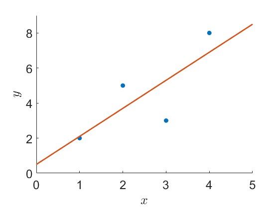
Example: Apply the least squares approach to the following observations.

\(x_{j}\)	1	2	3	4
\(y_{j}\)	2	5	3	8

Solution:

We form the following table,

\(x_{j}\)	\(y_{j}\)	\(x_{j}y_{j}\)	\(x_{j}^{2}\)
1	2	2	1
2	5	10	4
3	3	9	9
4	8	32	16
\(\sum_{j = 0}^{n} x_{j} = 10\)	\(\sum_{j = 0}^{n} y_{j} = 18\)	\(\sum_{j = 0}^{n} x_{j}y_{j} = 53\)	\(\sum_{j = 0}^{n} x_{j}^{2} = 30\)

Now, we need to solve the following linear system

\[\begin{equation*} \left[\begin{array}{cc} 4 & 10\\ 10 & 30 \end{array}\right] \left[\begin{array}{c}c_{0}\\ c_{1}\end{array}\right] = \left[\begin{array}{c} 18\\ 53 \end{array}\right]. \end{equation*}\]

This linear system can be expressed in the augmented matrix form

\[\begin{equation*} \left[\begin{array}{cc|c} 4 & 10 & 18\\ 10 & 30 & 53 \end{array}\right] \quad \Rightarrow \quad \left[\begin{array}{cc|r} 1 & 0 & \frac{1}{2}\\ 0 & 1 & \frac{8}{5} \end{array}\right] \end{equation*}\]

Thus, \(P(x) = \dfrac{1}{2} + \dfrac{8}{5}\,x\).