7.2. Matrix Factorization

7.2.1. LU decomposition

The \(LU\) decomposition decomposes a matrix into a lower triangular matrix \(L\) and an upper triangular matrix \(U\). Its main application is solving linear systems. Therefore, solving the linear system \(Ax = b\) where \(A\) is a \(n\times n\) matrix and \(x\) and \(b\) are vectors of length \(n\) can be as represented as follows.

\[\begin{align*}\label{C7_liner_eq} Ax=(LU)x=L(Ux)=b, \end{align*}\]

This is equivalent to

\[\begin{align*} \begin{cases} Ly = b,\\ Ux = y. \end{cases} \end{align*}\]

Solving the last two linear systems is equivalent to the forward elimination and back substitution, respectively.

Theorem

Let \(A = (a_{ij})\) be an \(n\times n\) matrix, where \(1\leq i,j \leq n\), and let all of its diagonal submatrices of order \(k\) be nonsingular. We can assert the existence of matrices \(L\) and \(U\) satisfying the following conditions: \(L\) is a lower triangular matrix with ones along its diagonal, \(U\) is an upper triangular matrix, and \(A = LU\) [Allaire, Kaber, Trabelsi, and Allaire, 2008, Atkinson, 2004, Khoury and Harder, 2016].

Let \(A\) be a square matrix. Then, \(A\) can be decomposed into \(L\) and \(U\) as follows,

\[\begin{align*} \begin{bmatrix}a_{11} & a_{12} & \dots & a_{1n} \\ a_{21} & a_{22} & \dots & a_{2n} \\ \vdots & \vdots & & \vdots \\ a_{n1} & a_{n2} & \dots & a_{nn} \end{bmatrix}= \begin{bmatrix}1 & 0 & \dots & 0 \\ l_{21} & 1 & \dots & 0 \\ \vdots & \vdots & & \vdots \\ l_{n1} & l_{n2} & \dots & 1 \end{bmatrix} \begin{bmatrix}u_{11} & u_{12} & \dots & u_{1n} \\ 0 & u_{22} & \dots & u_{2n} \\ \vdots & \vdots & & \vdots \\ 0 & 0 & \dots & u_{nn} \end{bmatrix}. \end{align*}\]

Observe that \(L\) is lower triangular and \(U\) upper triangular. Thus,

\[\begin{align*} a_{ij} = \sum_{k = 1}^{n} l_{ik} u_{kj} = \sum_{k = 1}^{\min(i,j)} l_{ik} u_{kj}, \quad 1\leq i,j\leq n. \end{align*}\]

Solving this system:

• Column 1. Set \(j = 1\) and for \(1\leq i\leq n\), we have,

\[\begin{align*} \begin{array}{lcl} a_{11} = l_{11}\,u_{11} & \Rightarrow & u_{11} = a_{11},\\ a_{21} = l_{21}\,u_{11}& \Rightarrow & l_{21} = u_{21}/a_{11},\\ \vdots & & \vdots\\ a_{n1} = l_{n1}\,u_{11}& \Rightarrow & l_{n1} = u_{n1}/a_{11}, \end{array} \end{align*}\]

• Column j. For a fixed \(j\) and for \(1\leq i\leq n\), we have,

\[\begin{align*} \begin{array}{lcl} a_{1j} = l_{11}\,u_{1j} & \Rightarrow & u_{1j} = a_{1j},\\ a_{21} = l_{21}\,u_{1j} + l_{22}\,u_{2j} & \Rightarrow & u_{2j} = a_{2j} - a_{21}\,a_{1j} ,\\ \vdots & & \vdots\\ a_{jj} = l_{j1}\,u_{1j} + \ldots + l_{jj}\,u_{jj} & \Rightarrow & u_{jj} = a_{jj} - \sum_{k = 1}^{j-1} l_{jk}\,u_{kj},\\ a_{j+1,j} = l_{j+1,1}\,u_{1j} + \ldots + l_{j+1,j}\,u_{jj} & \Rightarrow & l_{j+1,j} = \frac{1}{u_{jj}} \left( a_{j+1,j} - \sum_{k = 1}^{j-1} l_{j+1,k}\,u_{kj} \right),\\ \vdots & & \vdots\\ a_{nj} = l_{n,1}\,u_{1j} + \ldots + l_{nj}\,u_{jj} & \Rightarrow & l_{n,j} = \frac{1}{u_{jj}} \left( a_{nj} - \sum_{k = 1}^{j-1} l_{nk}\,u_{kj} \right). \end{array} \end{align*}\]

Thus, \(u_{ij}\) and \(l_{ij}\) can be identified as follows

\[\begin{align*} u_{ij} &= a_{ij} - \sum_{k=1}^{i-1} u_{kj}l_{ik},\\ l_{ij} &= \frac{1}{u_{jj}} \left(a_{ij} - \sum_{k=1}^{j-1} u_{kj}l_{ik} \right). \end{align*}\]

See [1] for the full derivation of this algorithm.

Python Code

import numpy as np

def myLU(A):
    '''
    Assuming that no row interchanges are required, this function
    calculates a unit lower triangular matrix L, and an upper
    triangular matrix U such that LU = A

    Parameters
    ----------
    A : numpy array
        DESCRIPTION. Matrix A

    Returns
    -------
    L : numpy array
        DESCRIPTION. Matrix L from A = LU
    U : numpy array
        DESCRIPTION. Matrix U from A = LU

    '''
    
    n = A.shape[1]
    # Consider U as a copy matrix A
    U = A.copy().astype(float)
    
    for j in range(0, n-1):
        U[j+1:n,j] = U[j+1:n,j]/U[j,j];
        for i in range(j+1, n):
            U[i,j+1:n] = U[i,j+1:n]-U[i,j]*U[j,j+1:n]
    L = np.tril(U,-1)+ np.eye(n, dtype=float)
    U = np.triu(U)
    return L, U

MATLAB Code

function [L,U] = myLU(A)
%{
Assuming that no row interchanges are required, this function
calculates a unit lower triangular matrix L, and an upper
triangular matrix U such that LU = A

Parameters
----------
A : array
    DESCRIPTION. Matrix A

Returns
-------
L : array
    DESCRIPTION. Matrix L from A = LU
U : array
    DESCRIPTION. Matrix U from A = LU
%}
n=length(A);
U = A;
for j=1:n-1
    U(j+1:n,j)= U(j+1:n,j)/U(j,j);
    for i=j+1:n
        U(i,j+1:n)=U(i,j+1:n)-U(i,j)*U(j,j+1:n);
    end
end
L = tril(U,-1)+eye(n,n);
U = triu(U);
end

import sys
sys.path.insert(0,'..')
import hd_tools as hd

Loading BokehJS ...

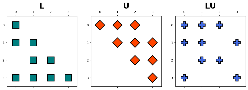
Example: Apply \(LU\) decomposition on the following matrix and identify \(L\) and \(U\).

\[\begin{align*}A = \left[\begin{array}{cccc} 7 & 3 & -1 & 2\\ 3 & 8 & 1 & -4\\ -1 & 1 & 4 & -1\\ 2 & -4 & -1 & 6 \end{array}\right].\end{align*}\]

Solution: We have,

import numpy as np
from hd_Matrix_Decomposition import myLU
from IPython.display import display, Latex
from sympy import init_session, init_printing, Matrix

A = np.array([ [7, 3, -1, 2], [3, 8, 1, -4], [-1, 1, 4, -1], [2, -4, -1, 6] ])
L, U = myLU(A)
display(Latex(r'L ='), Matrix(np.round(L, 2)))
display(Latex(r'U ='), Matrix(np.round(U, 2)))
display(Latex(r'LU ='), Matrix(L@U))

\[L =\]

\[\begin{split}\displaystyle \left[\begin{matrix}1.0 & 0 & 0 & 0\\0.43 & 1.0 & 0 & 0\\-0.14 & 0.21 & 1.0 & 0\\0.29 & -0.72 & 0.09 & 1.0\end{matrix}\right]\end{split}\]

\[U =\]

\[\begin{split}\displaystyle \left[\begin{matrix}7.0 & 3.0 & -1.0 & 2.0\\0 & 6.71 & 1.43 & -4.86\\0 & 0 & 3.55 & 0.32\\0 & 0 & 0 & 1.89\end{matrix}\right]\end{split}\]

\[LU =\]

\[\begin{split}\displaystyle \left[\begin{matrix}7.0 & 3.0 & -1.0 & 2.0\\3.0 & 8.0 & 1.0 & -4.0\\-1.0 & 1.0 & 4.0 & -1.0\\2.0 & -4.0 & -1.0 & 6.0\end{matrix}\right]\end{split}\]

hd.matrix_decomp_fig(mats = [L, U, L@U], labels = ['L', 'U', 'LU'])

Note that we could get similar results using Scipy LU function, scipy.linalg.lu.

import scipy.linalg as linalg
P, L, U = linalg.lu(A)
display(Latex(r'L ='), Matrix(np.round(L, 2)))
display(Latex(r'U ='), Matrix(np.round(U, 2)))

\[L =\]

\[\begin{split}\displaystyle \left[\begin{matrix}1.0 & 0 & 0 & 0\\0.43 & 1.0 & 0 & 0\\-0.14 & 0.21 & 1.0 & 0\\0.29 & -0.72 & 0.09 & 1.0\end{matrix}\right]\end{split}\]

\[U =\]

\[\begin{split}\displaystyle \left[\begin{matrix}7.0 & 3.0 & -1.0 & 2.0\\0 & 6.71 & 1.43 & -4.86\\0 & 0 & 3.55 & 0.32\\0 & 0 & 0 & 1.89\end{matrix}\right]\end{split}\]

Note that in the above algorithm \(P\) is a permutation matrix that can perform a partial and full pivoting.

7.2.2. Solving Linear systems using LU decomposition

We can solve the linear system \(Ax=b\) for \(x\) using \(LU\) decomposition. To demonstrate this, we use the following example,

Example: Solve the following linear system using \(LU\) decomposition.

\[\begin{align*} \begin{cases} 2\,x_{1}+x_{2}+x_{3}=7\\ x_{1}-2\,x_{2}+x_{4}=1\\ x_{2}+3\,x_{3}=11\\ 4\,x_{4}-x_{1}=15. \end{cases} \end{align*}\]

Solution:

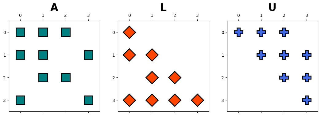
Let \(A=\left[\begin{array}{cccc}2 & 1 & 1 & 0\\ 1 & -2 & 0 & 1\\ 0 & 1 & 3 & 0\\ -1 & 0 & 0 & 4 \end{array}\right]\) and \(b=\left[\begin{array}{c} 7\\ 1\\ 11\\ 15 \end{array}\right]\).

Then, this linear system can be also expressed as follows,

\[\begin{align*} Ax=(LU)x=L(Ux)=b. \end{align*}\]

We have,

A = np.array([[2,1,1,0],[1,-2,0,1],[0,1,3,0],[-1,0,0,4]])
b = np.array([[7],[1],[11],[15]])
L, U = myLU(A)
display(Latex(r'L ='), Matrix(np.round(L, 2)))
display(Latex(r'U ='), Matrix(np.round(U, 2)))

\[L =\]

\[\begin{split}\displaystyle \left[\begin{matrix}1.0 & 0 & 0 & 0\\0.5 & 1.0 & 0 & 0\\0 & -0.4 & 1.0 & 0\\-0.5 & -0.2 & 0.14 & 1.0\end{matrix}\right]\end{split}\]

\[U =\]

\[\begin{split}\displaystyle \left[\begin{matrix}2.0 & 1.0 & 1.0 & 0\\0 & -2.5 & -0.5 & 1.0\\0 & 0 & 2.8 & 0.4\\0 & 0 & 0 & 4.14\end{matrix}\right]\end{split}\]

hd.matrix_decomp_fig(mats = [A, L, U], labels = ['A', 'L', 'U'])

Now, we can solve the following linear systems instead

\[\begin{align*} \begin{cases} Ly=b,\\ Ux=y. \end{cases}. \end{align*}\]

# solving Ly=b for y
y = linalg.solve(L, b)
display(Latex(r'y ='), Matrix(np.round(y, 2)))

\[y =\]

\[\begin{split}\displaystyle \left[\begin{matrix}7.0\\-2.5\\10.0\\16.57\end{matrix}\right]\end{split}\]

# solving Ux=y for x
x = linalg.solve(U, y)
display(Latex(r'x ='), Matrix(np.round(x, 2)))

\[x =\]

\[\begin{split}\displaystyle \left[\begin{matrix}1.0\\2.0\\3.0\\4.0\end{matrix}\right]\end{split}\]

Let’s now solve the linear system directly and compare the results.

x_new = linalg.solve(A, b)
display(Latex(r'x ='), Matrix(np.round(x_new, 2)))

\[x =\]

\[\begin{split}\displaystyle \left[\begin{matrix}1.0\\2.0\\3.0\\4.0\end{matrix}\right]\end{split}\]