Gaussian quadrature

5.5. Gaussian quadrature#

Gaussian quadrature selects the points in an optimal manner (instead of an equally-spaced way). Consequently, the nodes $x_j,~1\leq j \leq n$ in the interval [a, b] and coefficients $w_j,~1\leq j \leq n$, are determined to minimize the anticipated error conveyed in the approximation

(5.58)#\[\begin{equation}\label{gq_eq.01} \int_{-1}^{1}f(x)\,dx \approx \sum _{i=1}^{n} w_{i}f \left(x_i\right). \end{equation}\]

Whenever \hlg{$f(x)$ is a polynomial of degree (up to) $2n-1$, this approximation is exact [Burden and Faires, 2005]. Moreover, usually, these approximations are done using $[-1,~1]$ interval.

For example, for $f(x) = a_{0} + a_{1} x + a_{2}x^{2} + a_{3}x^{3}$ with $n=2$, we have,

(5.59)#\[\begin{align} \int_{-1}^{1} a_{0} + a_{1} x + a_{2}x^{2} + a_{3}x^{3} \,dx & = w_{1}\left(a_{0} + a_{1} x_{1} + a_{2}x_{1}^{2} + a_{3}x_{1}^{3}\right) \notag \\ & + w_{2}\left(a_{0} + a_{1} x_{2} + a_{2}x_{2}^{2} + a_{3}x_{2}^{3}\right). \end{align}\]

On the other hand, since

(5.60)#\[\begin{equation} \int ^b_a( f(x) \pm g(x))\,dx = \int^b _a f(x).dx \pm \int^b_ag(x)\,dx \end{equation}\]

and

(5.61)#\[\begin{align}\label{gq_eq.02} \int_{-1}^{1} a_{0} + a_{1} x + a_{2}x^{2} + a_{3}x^{3} \,dx &= a_{0} \int_{-1}^{1} 1 \,dx +a_{1} \int_{-1}^{1} x\,dx +a_{2} \int_{-1}^{1} x^{2} \,dx +a_{3} \int_{-1}^{1} x^{3} \,dx, \end{align}\]

we have,

(5.62)#\[\begin{align} {a_{0} \int_{-1}^{1} 1 \,dx}+ {a_{1} \int_{-1}^{1} x\,dx} &+ {a_{2} \int_{-1}^{1} x^{2} \,dx} + {a_{3} \int_{-1}^{1} x^{3} \,dx} = {a_{0}\left(w_{1} + w_{2}\right)} + {a_{1}\left(w_{1}x_{1} + w_{2}x_{2}\right)} \notag \\ & + {a_{2}\left(w_{1}x_{1}^{2} + w_{2}x_{2}^{2}\right)} +{a_{3}\left(w_{1}x_{1}^{3} + w_{2}x_{2}^{3}\right)}. \end{align}\]

Therefore, we need to identify $w_{1}$, $w_{2}$, $x_{1}$, and $x_{2}$ from the following system of equations,

(5.63)#\[\begin{align}\label{gq_eq.03} \begin{cases} {\displaystyle w_{1} + w_{2} = \int_{-1}^{1} 1 \,dx = 2,} \\ {\displaystyle w_{1}x_{1} + w_{2}x_{2} = \int_{-1}^{1} x \,dx = 0,} \\ {\displaystyle w_{1}x_{1}^{2} + w_{2}x_{2}^{2} = \int_{-1}^{1} x^{2} \,dx = \frac{2}{3},} \\ {\displaystyle w_{1}x_{1}^{3} + w_{2}x_{2}^{3} = \int_{-1}^{1} x^{3} \,dx = 0.} \end{cases} \end{align}\]

Solving this system of equations leads to $w_{1} = w_{2} = 1$ and $x_{1} = -\dfrac{\sqrt{3}}{3} = -x_{2}$. Hence,

(5.64)#\[\int _{-1}^{1}f(x)\,dx\approx f\left(-\frac{\sqrt{3}}{3}\right) + f\left(\frac{\sqrt{3}}{3}\right).\]

This formula (5.64) has a precision of 3. This it delivers the exact solution for any polynomial of degree 3 or less.

Python Code

import numpy as np

def TwoPointGaussian(f):
    '''
    Parameters
    ----------
    f : function 
        DESCRIPTION. A function. Here we use lambda functions

    Returns
    -------
    S : float
        DESCRIPTION. Numerical Integration of f(x) on [a,b]
        through TwoPointGaussian

    '''
    return f(-np.sqrt(3)/3) + f(np.sqrt(3)/3)

MATLAB Code

function [Int] = TwoPointGaussian(f)
%{
Parameters
----------
f : function 
    DESCRIPTION. A function. Here we use lambda functions

Returns
-------
S : float
    DESCRIPTION. Numerical Integration of f(x) on [a,b]
    through TwoPointGaussian

%}
Int = f(-sqrt(3)/3) + f(sqrt(3)/3);

First, we have

\[\begin{align*} \int _{1}^{-1}x^{2}\,dx = \frac{1}{3} x^{3}\Big|_{-1}^{1} = \frac{2}{3}. \end{align*}\]

from IPython.display import display, Latex
import sys
sys.path.insert(0,'..')
from hd_Numerical_Integration_Algorithms import TwoPointGaussian
Int = TwoPointGaussian(f = lambda x: x**2)
display(Latex('''\\left(-\\frac{\\sqrt{3}}{3}\\right) + f\\left(\\frac{\\sqrt{3}}{3}\\right) =  %.4f''' % Int))

\[\left(-\frac{\sqrt{3}}{3}\right) + f\left(\frac{\sqrt{3}}{3}\right) = 0.6667\]

Moreover, $$\int _{1}^{-1}x^{3} - x^{2} + 1\,dx =\frac{1}{4} x^{4}\Big|_{-1}^{1} - \frac{1}{3} x^{3}\Big|_{-1}^{1} + x\Big|_{-1}^{1}= \frac{4}{3}$$.

Trying this numerically,

Int = TwoPointGaussian(f = lambda x: x**3-x**2+1)
display(Latex('''\\left(-\\frac{\\sqrt{3}}{3}\\right) + f\\left(\\frac{\\sqrt{3}}{3}\\right) =  %.4f''' % Int))

5.5.1. Legendre polynomials#

The Legendre polynomials is a collection $\{P_0(x), P_1(x), \ldots , P_n(x), \ldots \}$ with properties [Burden and Faires, 2005]:

$P_n(x),~n\in \mathbb{N}$ is a monic (univariate) polynomial of degree $n$.
${\displaystyle \int_{-1}^{1} P(x)P_{n}(x)\,dx = 0}$ whenever $P(x)$ is a polynomial of degree less than $n$.

~\ \noindent Rodrigues’ formula provides a simple formulation for the Legendre polynomials \cite{hom2006, aratyn2006short}:

(5.65)#\[\begin{equation}\label{Rodrigues_forumula} P_{n}(x)={\frac {1}{2^{n}n!}}{\frac {d^{n}}{dx^{n}}}(x^{2}-1)^{n}\,. \end{equation}\]

This equation allows for the derivation of a large number of $P_{n}$ polynomials. The above also can be expressed as follows \cite{aratyn2006short},

(5.66)#\[\begin{equation} P_{n}(x)={\frac {1}{2^{n}}}\sum _{k=0}^{n}{\binom {n}{k}}^{2}(x-1)^{n-k}(x+1)^{k}. \end{equation}\]

The first few Legendre polynomials:

$P_{0}(x) = 1$,
$P_{1}(x) = x$,
$P_{2}(x) = \dfrac{1}{2} (3x^2 - 1)$,
$P_{3}(x) = \dfrac{1}{2} (5x^3 - 3x)$,
$P_{4}(x) = \dfrac{1}{8} (35x^4 - 30x^2 + 3)$,
$P_{5}(x) = \dfrac{1}{16} (63x^5 - 70x^3 + 15x)$,
$P_{6}(x) = \dfrac{1}{16} (231x^6 - 315x^4 + 105x^2 - 5)$,

In MATLAB, \href{https://www.mathworks.com/help/symbolic/sym.legendrep.html}{legendreP(n,x)} returns the $n$th degree Legendre polynomial at $x$. For example,

legendreP(3, x)

ans = (5x^3)/2 - (3x)/2

In Python, \href{https://docs.scipy.org/doc/scipy/reference/generated/scipy.special.legendre.html}{scipy} includes legendre polynomials. For example, to generate the 3rd-order Legendre polynomial:

from scipy.special import legendre
from numpy import poly1d
print(legendre(3))

Output: 3 2.5 x - 1.5 x

The following proposition is Theorem 4.7 from [Burden and Faires, 2005].

Theorem

Let $x_{1}$, $x_{2}$, \ldots , $x_{n}$ be the roots of the $n$th Legendre polynomial $P_n(x)$ and that for each $i = 1,~2,~\ldots,~n$, the numbers $w_{i}$ are defined as follows,

(5.67)#\[\begin{align}\label{gq_eq.05} w_{i} = \int_{-1}^{1} \prod\limits_{\substack{j = 1\\j \neq i}}^{n} \dfrac{x-x_{j}}{x_{i} - x_j}\,dx. \end{align}\]

Furthermore, if $P(x)$ is any polynomial of degree less than $2n$, then, the coefficient $w_i$ can be calculated using

(5.68)#\[\begin{align}\label{gq_eq.06} \int _{-1}^{1} P(x) \,dx = \sum _{i=1}^{n} w_{i}P \left(x_i \right). \end{align}\]

Proof: First, let’s assume that the degree of $P(x)$ is less than $n$. Then, we can express $P(x)$ in terms of $(n - 1)$st Lagrange coefficient polynomials with nodes at the roots of the $n$th Legendre polynomial $P_{n}(x)$. Note that, for this representation, the error term would include the $n$th derivative of $P(x)$. Since we assumed that $P(x)$ is of degree less than $n$, the $n$th derivative of $P(x)$ is 0, and this representation would be exact (why!?). Therefore,

(5.69)#\[\begin{equation} P(x) = \sum_{i = 1}^{n} P(x_{i})L_{i}(x) = \sum_{i = 1}^{n}\sum_{j = 1}^{j \neq i}\frac{x-x_{j}}{x_{i} - x_j}P(x_{i}) \end{equation}\]

and

(5.70)#\[\begin{align} \int _{-1}^{1} P(x) \,dx & = \int _{-1}^{1} \left[ \sum_{i = 1}^{n} \sum_{j = 1}^{j \neq i}\frac{x-x_{j}}{x_{i} - x_j}P(x_{i}) \right] \notag \\ & = \sum_{i = 1}^{n} \left[\int _{-1}^{1} \sum_{j = 1}^{j \neq i}\frac{x-x_{j}}{x_{i} - x_j}P(x_{i})\right] = \sum _{i=1}^{n} w_{i}P \left(x_i \right) \end{align}\]

Therefore, the result is true for polynomials of degree less than $n$.

Next, let’s assume a polynomial $P(x)$ of degree betweeb $n$ and $2n$. Also, divide $P(x)$ by the $n$th Legendre polynomial $P_n(x)$. This assumption can lead to two polynomials with less than degree $n$, $Q(x)$ and $R(x)$.

(5.71)#\[\begin{equation}\label{LegendreP_eq01} P(x) = Q(x) P_n(x) + R(x). \end{equation}\]

Observe that $x_{i}$ is a root of $P_n(x)$ for each $i = 1, 2, \ldots , n$. Therefore,

(5.72)#\[\begin{equation}\label{GQ_Question} P(x_{i}) = Q(x_{i}) P_n(x_{i}) + R(x_{i}) = R(x_{i}). \end{equation}\]

Now, since the degree of the polynomial $Q(x)$ is less than $n$, so (by Legendre property (2)),

(5.73)#\[\begin{equation}\label{LegendreP_eq02} \int _{-1}^{1}Q(x) P_{n}(x)\,dx = 0. \end{equation}\]

Furthermore, since $R(x)$ is a polynomial of degree less than $n$, we have,

(5.74)#\[\begin{equation}\label{LegendreP_eq03} \int _{-1}^{1}R(x)\,dx = \sum_{i = 1}^{n}w_{i}R(x_{i}). \end{equation}\]

Therefore

(5.75)#\[\begin{equation} \int _{-1}^{1}P(x)\,dx = \int _{-1}^{1} \left(Q(x) P_n(x) + R(x)\right)\,dx = \int _{-1}^{1}R(x)\,dx = \sum_{i = 1}^{n}w_{i}R(x_{i}) = \sum_{i = 1}^{n}w_{i}P(x_{i}). \end{equation}\]

These coefficients can be calculated using numpy leggauss function. For example, for polynomials of degree $n$ with $n=1,2\ldots,8$, we have

import pandas as pd
pd.options.mode.chained_assignment = None
Table = pd.DataFrame(columns = ['n', 'xi', 'wi'])
N = 9
Table['n'] = np.arange(1, N)
for n in range(Table.shape[0]):
     Table['xi'][n], Table['wi'][n] = np.round(np.polynomial.legendre.leggauss(Table.loc[n, 'n']), 6)
    
display(Table.style.set_properties(subset=['n'],
                   **{'background-color': 'Honeydew', 'color': 'Black','border-color': 'DarkGreen'}).hide(axis='index'))

5.5.2. Change of interval#

To approximate the integral of a function over an interval $[a,~b]$, this interval should be transformed into an integral over $[-1,~1]$ before using the Gaussian quadrature rule. This can be done as follows [Bojanov and Petrov, 2001, Wendroff, 2014]:

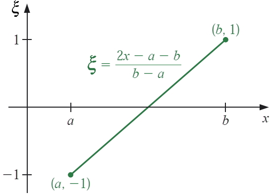
(5.76)#\[\begin{equation}\label{gq_eq.07} \int _{a}^{b}f(x)\,dx={\frac {b-a}{2}}\int _{-1}^{1}f\left({\frac {b-a}{2}}\xi +{\frac {a+b}{2}}\right)\,d\xi. \end{equation}\]

../_images/GQ_Figure.jpg — Fig. 5.4 Using the change of variables, an integral over $[a,~b]$ can be translated into an integral over $[-1, 1]$. Figure is from [Burden and Faires, 2005] with minor modifications.#

Now, a $n$-point Gaussian quadrature over an interval $[a, b]$ can be expressed as follows:

(5.77)#\[\begin{equation}\label{gq_eq.08} {\int _{a}^{b}f(t)\,dt\approx {\frac {b-a}{2}}\sum _{i=1}^{n}w_{i}f\left({\frac {b-a}{2}}x _{i}+{\frac {a+b}{2}}\right).} \end{equation}\]

Python Code

def GaussQuadrature(f, a, b, n):
    '''
    Parameters
    ----------
    f : function 
        DESCRIPTION. A function. Here we use lambda functions
    a : float
        DESCRIPTION. a is the left side of interval [a, b]
    b : float
        DESCRIPTION. b is the right side of interval [a, b]
    N : int
        DESCRIPTION. Number of xn points

    Returns
    -------
    S : float
        DESCRIPTION. Numerical Integration of f(x) on [a,b]
        through GaussQuadrature rule

    '''
    x, w = np.polynomial.legendre.leggauss(n)
    return 0.5*(b-a)*sum(w*f(0.5*(b-a)*x+0.5*(b+a)))

MATLAB Code

import sys
sys.path.insert(0,'..')
import hd_tools as hd

Example: Approximate each integration using 2-point and 3-point Gaussian quadrature rules and the change of interval formula

a. \task ${\displaystyle \int_{0}^{2}x^{2}\,dx}$,
b. \task ${\displaystyle \int_{-2}^{4}(x^{3} - x^{2} + 1)\,dx}$.

a. First, note that,

\[\begin{equation*} \int_{0}^{2} x^{2}\,dx = \frac{1}{3} x^{3}\Big|_{0}^{2} = \frac{8}{3}. \end{equation*}\]

Observe that the degree $x^{2}$ is less than \hl{$2n$} and we know that formula \eqref{gq_eq.04} would provide the exact value. Using the 2-point Gaussian quadrature rule, \hlg{$n=2$}, we have,

\[\begin{align*} \int_{0}^{2}t^{2}\,dt & = \frac{b-a}{2}\left[ w_{0}f\left({\frac {b-a}{2}}x_{0}+{\frac {a+b}{2}}\right) + w_{1}f\left({\frac {b-a}{2}}x_{1}+{\frac {a+b}{2}}\right) \right] \\ & = \frac{2-0}{2}\left[ w_{0}f\left({\frac {2-0}{2}}x_{0}+{\frac {2+0}{2}}\right) + w_{1}f\left({\frac {2-0}{2}}x_{1}+{\frac {2+0}{2}}\right) \right] \\ & = w_{0}f\left( x_{0} + 1\right) + w_{1}f\left( x_{1} + 1 \right). \end{align*}\]

Now, using Table \ref{Table_Legendre_coefficients}

\[\begin{align*} \int_{0}^{2}t^{2}\,dt & = f\left(-\frac{\sqrt{3}}{3} + 1\right) + f\left(\frac{\sqrt{3}}{3} + 1\right) = \left(-\frac{\sqrt{3}}{3} + 1\right)^2 + \left(\frac{\sqrt{3}}{3} + 1\right)^2 \\ & = \frac{4}{3}-\frac{2\,\sqrt{3}}{3} + \frac{2\,\sqrt{3}}{3}+\frac{4}{3} = \frac{8}{3} \end{align*}\]

Using the 3-point Gaussian quadrature rule, \hlg{$n=3$}, similarly, the degree of the polynomial is 2 and it is less than \hl{$2n$}. Now, using Table \ref{Table_Legendre_coefficients}, we have,

\[\begin{align*} \int_{0}^{2} t^{2}\,dt & = \frac{b-a}{2}\left[ w_{0}f\left({\frac {b-a}{2}}x_{0}+{\frac {a+b}{2}}\right) + w_{1}f\left({\frac {b-a}{2}}x_{1}+{\frac {a+b}{2}}\right) \right. \\ & \left. + w_{2}f\left({\frac {b-a}{2}}x_{2}+{\frac {a+b}{2}}\right) \right] \\ & = \frac{2-0}{2}\left[ w_{0}f\left({\frac {2-0}{2}}x_{0}+{\frac {2+0}{2}}\right) + w_{1}f\left({\frac {2-0}{2}}x_{0}+{\frac {2+0}{2}}\right) \right. \\ & \left. + w_{2}f\left({\frac {2-0}{2}}x_{0}+{\frac {2+0}{2}}\right) \right] \\ & = w_{0}f\left(x_{0} + 1\right) + w_{1}f\left( x_{1} + 1 \right) + w_{2}f\left( x_{2} + 1 \right) \\ & =\dfrac {5}{9}f\left( -\sqrt{\dfrac {3}{5}} + 1\right) + \dfrac {8}{9}f\left( 0 + 1 \right) + \dfrac {5}{9}f\left(\sqrt{\dfrac {3}{5}} + 1 \right) = \frac{8}{3}. \end{align*}\]

b. Similarly,

\[\begin{align*} \int_{-2}^{4} t^{3} - t^{2} + 1\,dt=\frac{1}{4} x^{4}\Big|_{-2}^{4}- \frac{1}{3} x^{3}\Big|_{-2}^{4}+ x\Big|_{-2}^{4}= 42. \end{align*}\]

Using the 2-point Gaussian quadrature rule, the degree of $x^{3} - x^{2} + 1$, 3 is less than $2n$, therefore, the approximation would be, in fact, exact. We have,

\[\begin{align*} \int_{0}^{2}t^{2}\,dt & = \frac{b-a}{2}\left[ w_{0}f\left({\frac {b-a}{2}}x_{0}+{\frac {a+b}{2}}\right) + w_{1}f\left({\frac {b-a}{2}}x_{1}+{\frac {a+b}{2}}\right) \right] \\ & = \frac{4-(-2)}{2}\left[ w_{0}f\left({\frac {4-(-2)}{2}}x_{0}+{\frac {4+(-2)}{2}}\right) + w_{1}f\left({\frac {4-(-2)}{2}}x_{1}+{\frac {4+(-2)}{2}}\right) \right] \\ & = 3\,w_{0}f\left( 3\,x_{0} + 1\right) + 3\,w_{1}f\left( 3\,x_{1} + 1 \right) \\ & = 3f\left(-3\,\frac{\sqrt{3}}{3} + 1\right) + 3f\left(3\,\frac{\sqrt{3}}{3} + 1\right) = 42. \end{align*}\]

Using the 3-point Gaussian quadrature rule, \hlg{$n=3$}, likewise, the degree of $x^{3} - x^{2} + 1$ is 3 and the approximation would be exact. The exact:

\[\begin{align*} \int_{-2}^{4} t^{3} - t^{2} + 1\,dt & = \frac{b-a}{2}\left[ w_{0}f\left({\frac {b-a}{2}}x_{0}+{\frac {a+b}{2}}\right) + w_{1}f\left({\frac {b-a}{2}}x_{1}+{\frac {a+b}{2}}\right) \right. \\ & \left. + w_{2}f\left({\frac {b-a}{2}}x_{2}+{\frac {a+b}{2}}\right) \right] \\ & = \frac{4-(-2)}{2}\left[ w_{0}f\left({\frac {4-(-2)}{2}}x_{0}+{\frac {2+0}{2}}\right) + w_{1}f\left({\frac {4-(-2)}{2}}x_{0}+{\frac {4+(-2)}{2}}\right) \right. \\ & \left. + w_{2}f\left({\frac {4-(-2)}{2}}x_{0}+{\frac {4+(-2)}{2}}\right) \right] \\ & = 3\,w_{0}f\left(3\,x_{0} + 1\right) + 3\,w_{1}f\left(3\,x_{1} + 1 \right) + 3\,w_{2}f\left(3\,x_{2} + 1 \right) = 42. \end{align*}\]

from hd_Numerical_Integration_Algorithms import GaussQuadrature 
for n in range(2, 5):
    print('Gaussian quadrature using the %i-point = %.8f' % (n, GaussQuadrature(f = lambda x : x**2, a = 0, b = 1, n = n)))

Gaussian quadrature

Contents

5.5. Gaussian quadrature#

5.5.1. Legendre polynomials#

5.5.2. Change of interval#