7.3. Cholesky factorization

Definition: The Transpose of a Matrix

Transpose of a matrix is formed by turning rows into columns and vice versa. For a matrix \(A\), we denote the transpose of \(A\) by \(A^T\).

Definition: Symmetric and Skew Symmetric Matrices

An \(n\times n\) matrix \(A\) is

• Symmetric if \(A = A^T\).

• Skew-symmetric if \(A = -A^T\).

Definition: Positive Definite

An \(n\times n\) complex matrix \(A\) is positive definite if

\[\begin{align*} x^TAx > 0, \end{align*}\]

for all nonzero vectors x in \(\mathbb{R}^n\).

Theorem

Assume that \(A\) is a real and symmetric positive definite matrix. Then, a unique real lower triangular matrix B with positive diagonal entries exists such that

\[\begin{align*} A = BB^T, \end{align*}\]

where \(B^T\) denotes the conjugate transpose of \(B\).

Furthermore, We have,

\[\begin{align*} \begin{bmatrix}a_{11} & a_{12} & \dots & a_{1n} \\ a_{21} & a_{22} & \dots & a_{2n} \\ \vdots & \vdots & & \vdots \\ a_{n1} & a_{n2} & \dots & a_{nn} \end{bmatrix}= \begin{bmatrix}b_{11} & 0 & \dots & 0 \\ b_{21} & b_{22} & \dots & 0 \\ \vdots & \vdots & & \vdots \\ b_{n1} & b_{n2} & \dots & b_{nn} \end{bmatrix} \begin{bmatrix}b_{11} & b_{12} & \dots & b_{1n} \\ 0 & b_{22} & \dots & b_{2n} \\ \vdots & \vdots & & \vdots \\ 0 & 0 & \dots & b_{nn} \end{bmatrix}. \end{align*}\]

Observe that \(L\) is lower triangular and \(U\) upper triangular. Thus,

\[\begin{align*} a_{ij} = \sum_{k = 1}^{n} b_{ik} b_{jk} = \sum_{k = 1}^{\min(i,j)} b_{ik} b_{jk}, \quad 1\leq i,j\leq n. \end{align*}\]

Solving this system:

• Column 1. Set \(j = 1\) and for \(1\leq i\leq n\), we have,

\[\begin{align*} \begin{array}{lcl} a_{11} = (b_{11})^2 & \Rightarrow & b_{11} = \sqrt{a_{11}},\\ a_{21} = b_{11}\,b_{21}& \Rightarrow & b_{21} = a_{21}/b_{11},\\ \vdots & & \vdots\\ a_{n1} = b_{11}\,b_{n1}& \Rightarrow & b_{n1} = a_{n1}/b_{11}, \end{array} \end{align*}\]

• Column j. For a fixed \(j\) and for \(1\leq i\leq n\), we have,

\[\begin{align*} \begin{array}{lcl} a_{jj} = (b_{j1})^2 + (b_{j2})^2 + \ldots + (b_{jj})^2 & \Rightarrow & b_{jj} = \sqrt{a_{jj} - \sum_{k = 1}^{j-1} (b_{jk})^2},\\ a_{j+1,j} = b_{j1}\,b_{j+1,1} + \ldots + b_{jj}\,b_{j+1,j} & \Rightarrow & b_{j+1,j} = \frac{1}{b_{jj}} \left( a_{j+1,j} - \sum_{k = 1}^{j-1} b_{jk}\,b_{j+1,k} \right),\\ \vdots & & \vdots\\ a_{nj} = b_{j,1}\,b_{n1} + \ldots + b_{jj}\,b_{nj} & \Rightarrow & b_{nj} = \frac{1}{b_{jj}} \left( a_{nj} - \sum_{k = 1}^{j-1} b_{jk}\,b_{nk} \right). \end{array} \end{align*}\]

Thus,

\[\begin{align*} b_{j,j} &={\sqrt {a_{j,j}-\sum _{k=1}^{j-1}b_{j,k}^{2}}},\\ b_{i,j}&={\frac {1}{a_{j,j}}}\left(a_{i,j}-\sum _{k=1}^{j-1}b_{i,k}b_{j,k}\right)\quad {\text{for }}i>j. \end{align*}\]

See [Allaire, Kaber, Trabelsi, and Allaire, 2008, Khoury and Harder, 2016] for the full derivation of this algorithm.

Python Code

import numpy as np

def myCholesky(A):
    '''
    Assuming that the matrix A is symmetric and positive definite,
    this function calculates a lower triangular matrix G with positive
    diagonal entries, such that A = BB^T

    Parameters
    ----------
    A : numpy array
        DESCRIPTION. Matrix A

    Returns
    -------
    B : numpy array
        DESCRIPTION. Matrix B from A = BB*

    '''
    
    n = A.shape[1]
    B = np.zeros([n, n], dtype=float);
    B[0,0] = np.sqrt(A[0,0]);
    B[1:n, 0]= A[1:n,0] / B[0,0];
    for j in range(1, n):
        B[j,j] = np.sqrt(A[j,j]- np.dot(B[j, 0:j], B[j, 0:j]))
        for i in range(j+1, n):
            B[i,j]=(A[i,j] - np.dot(B[i, 0:j],B[j, 0:j]))/B[j,j]
    return B   

MATLAB Code

function [B] = myCholesky(A)
%{
Assuming that the matrix A is symmetric and positive definite,
this function calculates a lower triangular matrix G with positive
diagonal entries, such that A = BB^T

Parameters
----------
A : numpy array
    DESCRIPTION. Matrix A

Returns
-------
B : numpy array
    DESCRIPTION. Matrix B from A = BB*
%}

B = zeros(n,n);
B(1,1)=sqrt(A(1,1));
B(2:n,1)=A(2:n,1)/B(1,1);
for j=2:n
    B(j,j)=sqrt(A(j,j)-dot(B(j,1:j-1),B(j,1:j-1)));
    for i=j+1:n
        B(i,j)=(A(i,j)-dot(B(i,1:j-1),B(j,1:j-1)))/B(j,j);
    end
end

import sys
sys.path.insert(0,'..')
import hd_tools as hd

Loading BokehJS ...

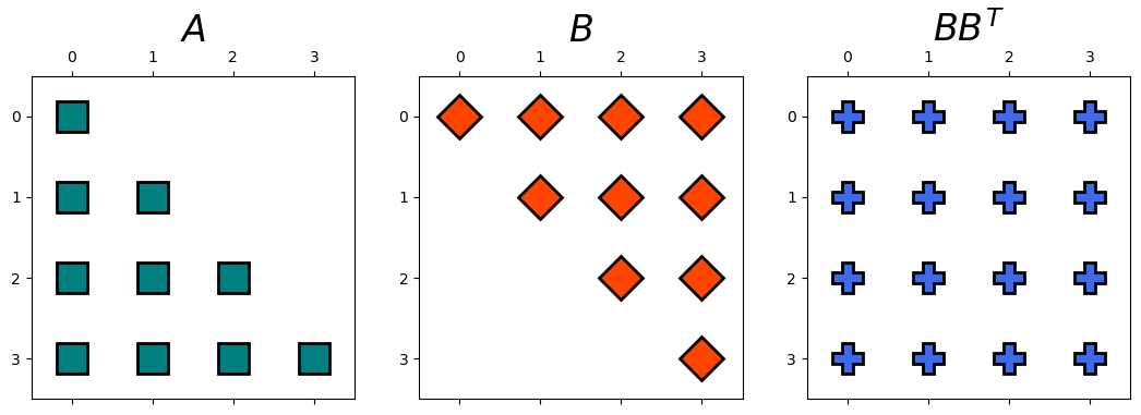
Example: Apply Cholesky decomposition on the following matrix and identify \(B\).

\[\begin{align*}A = \left[\begin{array}{cccc} 7 & 3 & -1 & 2\\ 3 & 8 & 1 & -4\\ -1 & 1 & 4 & -1\\ 2 & -4 & -1 & 6 \end{array}\right].\end{align*}\]

Solution: We have,

import numpy as np
from hd_Matrix_Decomposition import myCholesky
from IPython.display import display, Latex
from sympy import init_session, init_printing, Matrix

A = np.array([ [7, 3, -1, 2], [3, 8, 1, -4], [-1, 1, 4, -1], [2, -4, -1, 6] ])
B = myCholesky(A)

display(Latex(r'A ='), Matrix(A))
display(Latex(r'B ='), Matrix(np.round(B, 2)))
display(Latex(r'B  B^T ='), Matrix(np.round(np.matmul(B,B.T), 2)))

\[A =\]

\[\begin{split}\displaystyle \left[\begin{matrix}7 & 3 & -1 & 2\\3 & 8 & 1 & -4\\-1 & 1 & 4 & -1\\2 & -4 & -1 & 6\end{matrix}\right]\end{split}\]

\[B =\]

\[\begin{split}\displaystyle \left[\begin{matrix}2.65 & 0 & 0 & 0\\1.13 & 2.59 & 0 & 0\\-0.38 & 0.55 & 1.88 & 0\\0.76 & -1.87 & 0.17 & 1.37\end{matrix}\right]\end{split}\]

\[B B^T =\]

\[\begin{split}\displaystyle \left[\begin{matrix}7.0 & 3.0 & -1.0 & 2.0\\3.0 & 8.0 & 1.0 & -4.0\\-1.0 & 1.0 & 4.0 & -1.0\\2.0 & -4.0 & -1.0 & 6.0\end{matrix}\right]\end{split}\]

hd.matrix_decomp_fig(mats = [B, B.T, np.round(np.matmul(B,B.T), 2)], labels = ['$A$', '$B$', '$B  B^T$'])

Note that we could get a similar results using function, numpy.linalg.cholesky.

import scipy.linalg as linalg
B = np.linalg.cholesky(A)
display(Latex(r'B ='), Matrix(np.round(B, 2)))

\[B =\]

\[\begin{split}\displaystyle \left[\begin{matrix}2.65 & 0 & 0 & 0\\1.13 & 2.59 & 0 & 0\\-0.38 & 0.55 & 1.88 & 0\\0.76 & -1.87 & 0.17 & 1.37\end{matrix}\right]\end{split}\]

7.3.1. Solving Linear systems using Cholesky factorization

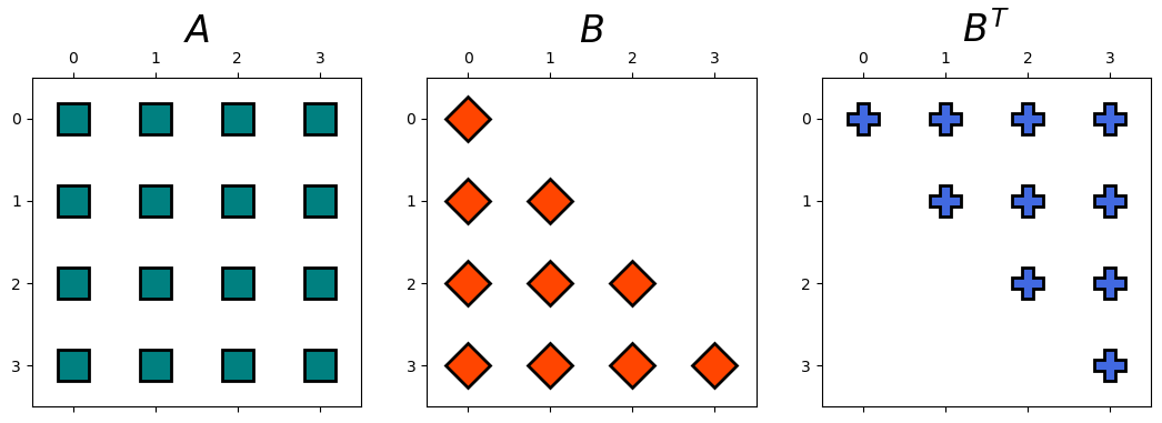
We can solve the linear system \(Ax=b\) for \(x\) using Cholesky decomposition. To demonstrate this, we use the following example,

Example: Solve the following linear system using Cholesky decomposition.

\[\begin{align*} \begin{cases} 7\,x_{1}+3\,x_{2}-x_{3}+2\,x_{4}=18\\ 3\,x_{1}+8\,x_{2}+x_{3}-4\,x_{4}=6\\ x_{2}-x_{1}+4\,x_{3}-x_{4}=9\\ 2\,x_{1}-4\,x_{2}-x_{3}+6\,x_{4}=15 \end{cases} \end{align*}\]

Solution:

Let \(A=\left[\begin{array}{cccc} 7 & 3 & -1 & 2\\ 3 & 8 & 1 & -4\\ -1 & 1 & 4 & -1\\ 2 & -4 & -1 & 6 \end{array}\right]\) and \(b=\left[\begin{array}{c} 18\\ 6\\ 9\\ 15 \end{array}\right]\). Then, this linear system can be also expressed as follows,

\[\begin{align*} Ax=(BB^T)x=B(B^Tx)=b. \end{align*}\]

We have,

A = np.array([ [7, 3, -1, 2], [3, 8, 1, -4], [-1, 1, 4, -1], [2, -4, -1, 6] ])
b = np.array([[18],[ 6],[ 9],[15]])
B = myCholesky(A)
display(Latex(r'B ='), Matrix(np.round(B, 2)))

\[B =\]

\[\begin{split}\displaystyle \left[\begin{matrix}2.65 & 0 & 0 & 0\\1.13 & 2.59 & 0 & 0\\-0.38 & 0.55 & 1.88 & 0\\0.76 & -1.87 & 0.17 & 1.37\end{matrix}\right]\end{split}\]

hd.matrix_decomp_fig(mats = [A, B, B.T], labels = ['$A$', '$B$', '$B^T$'])

Now we can solve the following linear systems instead

\[\begin{align*}\begin{cases}By=b,\\ B^Tx=y.\end{cases}\end{align*}\]

# solving y
y = np.linalg.solve(B, b)
display(Latex(r'y ='), Matrix(np.round(y, 2)))

\[y =\]

\[\begin{split}\displaystyle \left[\begin{matrix}6.8\\-0.66\\6.33\\5.49\end{matrix}\right]\end{split}\]

# solving x
x = np.linalg.solve(B.T, y)
display(Latex(r'x ='), Matrix(np.round(x, 2)))

\[x =\]

\[\begin{split}\displaystyle \left[\begin{matrix}1.0\\2.0\\3.0\\4.0\end{matrix}\right]\end{split}\]

Let’s now solve the linear system directly and compare the results.

x_new = linalg.solve(A, b)
display(Latex(r'x ='), Matrix(np.round(x_new, 2)))

\[x =\]

\[\begin{split}\displaystyle \left[\begin{matrix}1.0\\2.0\\3.0\\4.0\end{matrix}\right]\end{split}\]