3.2. Vandermonde Method#
3.2.1. Univariate Polynomials#
Consider a distinct set of \(n + 1\) data points (no two \(x_{j}\)s are the same)
where
for some \(g\in C[a,b]\), and assume that
interpolates these points. This means
In other words,
This can be expressed as the following linear system of equations,
The matrix containing the values of the variables of the polynomial is called the \textbf{Vandermonde matrix}:
Let \(\textbf{c} = \begin{bmatrix}c_{0} & c_{1} & c_{2} & \dots & c_{n}\end{bmatrix}^T\) and \(\textbf{y} = \begin{bmatrix}y_{0} & y_{1} & y_{2} & \dots &y_{n}\end{bmatrix}^T\). We can find \(c_{0}\), \(c_{1}\), \(c_{2}\), \dots, \(c_{n}\) by solving
for \(\textbf{c}\).
Example: Consider the data points \((-2,1)\), \((0,1)\), \((2,9)\), \((3,16)\) . Find an interpolating polynomial \(p(x)\) of degree at most three, and estimate the value of \(p(1)\).
Solution: We like to identify
in a way that \(P_{3}(-2)=1\), \(P_{3}(0)=1\), \(P_{3}(2)=9\) and \(P_{3}(3)=16\).
We can substitute the known values in for \(x\) and solve for \(c_0\), \(c_1\), \(c_2\) and \(c_3\). Using the given points, the system of equations is
Observe that
The augmented matrix:
In Reduced Row Echelon Form (RREF):
Therefore, \(c_0 = 1\), \(c_1 = 2\) , \(c_2 = 1\), \(c_3 = 0\) and \(P_{3}(x) = x^2+2\,x+1\) . To estimate the value of \(p(1)\), we compute
import numpy as np

def VanderCoefs(xn, yn):
    '''
    xn : list/array
        DESCRIPTION. a list/array consisting points x0, x1, x2,... ,xn
    yn : list/array
        DESCRIPTION. a list/array consisting points
        y0 = f(x0), y1 = f(x1),... ,yn = f(xn)
    Returns
    -------
    cn : float
        DESCRIPTION. Vandermonde method coefficients
    '''
    n = len(xn)
    V = np.zeros((n, n), dtype = float)
    P = np.arange(n)
    for i in range(n):
        V[i, :] = xn[i]**P
    cn = np.linalg.solve(V, yn)
    return cn
function [cn] = VanderCoefs(xn, yn)
%{
xn : list/array
    DESCRIPTION. a list/array consisting points x0, x1, x2,... ,xn
yn : list/array
    DESCRIPTION. a list/array consisting points
    y0 = f(x0), y1 = f(x1),... ,yn = f(xn)
Returns
-------
cn : float
    DESCRIPTION. Vandermonde method coefficients
%}
n = length(xn);
V = zeros(n, n);
P = 0:(n-1);
for i = 1:n
    V(i, :) = xn(i).^P;
end
cn = linsolve(V,yn');
end
Example: In the previous Example, use VanderCoefs functions to identify Vandermonde method coefficients.
# This part is used for producing tables and figures
import sys
sys.path.insert(0,'..')
import hd_tools as hd
We use numpy polyval to form a polynomial.
import numpy as np
from hd_Interpolation_Algorithms import VanderCoefs

# A set of distinct points
xn = np.array ([-2, 0, 2, 3])
yn = np.array ([1, 1, 9, 16])
# Vandermonde method coefficients
cn = VanderCoefs(xn, yn)
x = np.linspace(xn.min()-1 , xn.max()+1 , 100)
y = np.polyval(np.flip(cn), x)
# Plots
hd.interpolation_method_plot(xn, yn, x, y, title = 'Vandermonde Method (Univariate Polynomials)')
3.2.2. Univariate General Functions#
In this method, instead of using just a polynomial, the desired functions \(f_{n}\) can be used. Therefore, for a distinct set of \(n + 1\) data points (no two \(x_{j}\)s are the same)
where
for some \(g\in C[a,b]\), and the following general form,
interpolates these points. This means \(P(x_i ) = y_i\) for \(i = 0, 1, 2, \ldots, n\). In other words,
This can be expressed as a system of equations. Thus,
and the Vandermonde Matrix:
def VanderCoefsGen(xn, yn, fn = False):
    '''
    xn : list/array
        DESCRIPTION. a list/array consisting points x0, x1, x2,... ,xn
    yn : list/array
        DESCRIPTION. a list/array consisting points
        y0 = f(x0), y1 = f(x1),... ,yn = f(xn)
    fn : a multi-output function
        base-functions for Vandermonde method
    Returns
    -------
    cn : float
        DESCRIPTION. Vandermonde method coefficients
    '''
    if not fn:
        fn = lambda x: x**np.arange(len(xn))
    n = len(xn)
    V = np.zeros((n, n), dtype = float)
    for i in range(n):
        V[i, :] = fn(xn[i])
    cn = np.linalg.solve(V, yn)
    return cn
Example: Consider the following data points
Construct an interpolating polynomial using Vandermonde method coefficients that use all this data. For \(f_n\) functions use
a) \(\left\{1,~x,x^2,\ldots,x^n\right\}\) as \(f_n\) functions,
b) \(\left\{\cos(x),~\cos(2x),~\cos(3x),\ldots,~\cos(nx)\right\}\) as \(f_n\) functions.
Solution:
a. This would be similar to the method discussed in Section \ref{Vandermonde_Univar}. Note that here \(n=5\), and the Vandermonde matrix corresponding to \(\left\{1,~x,~x^2,~x^3,~x^4,~x^5 \right\}\) can be found as follows,
Now, we can solve \(\textbf{V}\textbf{c} = \textbf{y}\) to find \(\textbf{c}\). Therefore,
Therefore,
b. In this case, we have,
Using \(\textbf{V}\textbf{c} = \textbf{y}\), we can find \(\textbf{c}\) as follows (using \(\textbf{c} = \textbf{V}^{-1}y\)):
\vspace{-0.5cm} Therefore,
We can also try parts (a) and (b) of this Example in Python.
from hd_Interpolation_Algorithms import VanderCoefsGen

# A set of distinct points
xn = np.array ([1 ,2 ,3 ,4 ,5 , 6])
yn = np.array ([-3 ,0 ,-1 ,2 ,1 , 4])
# Vandermonde method coefficients
cn = VanderCoefsGen(xn, yn)
x = np.linspace(xn.min()-1 , xn.max()+1 , 100)
y = np.polyval(np.flip(cn), x)
# Plots
hd.interpolation_method_plot(xn, yn, x, y, title = 'Vandermonde Method (Univariate Polynomials)')
For the above example, we can use \(\left\{\cos(x),~\cos(2x),~\cos(3x),\ldots,~\cos(nx)\right\}\) as \(f_n\) functions and use the Vandermonde Method.
# A set of distinct points
xn = np.array ([1 ,2 ,3 ,4 ,5 , 6])
yn = np.array ([-3 ,0 ,-1 ,2 ,1 , 4])
fn = lambda x: np.array([np.cos(n*x) for n in range(len(xn))])
# Vandermonde method coefficients
cn = VanderCoefsGen(xn, yn, fn)
x = np.linspace(xn.min()-1 , xn.max()+1 , 100)
y = (cn.reshape(1, len(cn))@fn(x)).flatten()
# Plots
hd.interpolation_method_plot(xn, yn, x, y, title = 'Vandermonde Method (Univariate General Functions)')
3.2.3. Multivariate General Functions#
Vandermonde’s method can be extended for the interpolation of multidimensional functions. For example, in three-dimensional space, for distinct points
we have
where \(f_{n}\) are desired functions. Similarly, we can form a linear system to find \(c_{0}\), \(c_{1}\),\dots \(c_{n}\). Thus,
which means,
This can be expressed as a system of equations. Thus,
and the Vandermonde Matrix:
def VanderCoefs3D(xn, yn, zn, fn):
    '''
    Parameters
    ----------
    xn : list/array
        DESCRIPTION. a list/array consisting points x0, x1, x2,... ,xn
    yn : list/array
        DESCRIPTION. a list/array consisting points y0, y1,... ,yn
    zn : list/array
        DESCRIPTION. a list/array consisting points
        z0 = f(x0,y0), z1 = f(x1,y1),... ,zn = f(xn,yn)
    fn : a multi-output function
        base-functions for Vandermonde method
    Returns
    -------
    cn : float
        DESCRIPTION. Vandermonde method coefficients

    '''
    V = np.zeros((len(xn), len(xn)), dtype = float)
    for i in range(len(xn)):
        V[i, :] = fn(xn[i], yn[i])
    cn = np.linalg.solve(V, zn)
    return cn
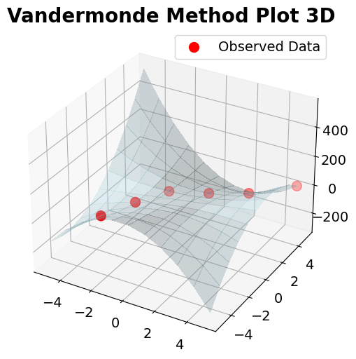
Example: Consider the following data points
Construct an interpolating polynomial using Vandermonde method coefficients that use all this data. For \(f_n\) functions use \(\{1, x, y, x\,y, x^2\,y, x\,y^2\}\).
Solution:
Here, using \(\{1,~x,~y,~x\,y,~x^2\,y,~x\,y^2\}\) we have,
Then, using \(\textbf{V}\textbf{c} = \textbf{z}\), we can find \(\textbf{c}\).
This means,
To verify this polynomial, it is enough to check
We also, could express \(\textbf{c}\) in the following format:
However, there will be some representation error as, for example,
Then using (3.13), we get \(-11\) while using (3.14), we get \(-11.000500000000009\). This difference is due the representation difference.
We can try this example in Python.
from hd_Interpolation_Algorithms import VanderCoefs3D

# A set of distinct points
xn = np.array ([-3, -2, -1, 1, 3, 5])
yn = np.array ([-3, -1, 1, 2, 3, 5])
zn = np.array ([-11 ,4 , 2 , -4 , 5, 10])

fn = lambda x, y: np.array([1, x, y, x*y, (x**2)*y, x*(y**2)])
cn = VanderCoefs3D(xn, yn, zn, fn)
# Vandermonde_Method_Plot_3D(xn, yn, zn, cn, fn)

import matplotlib.pyplot as plt

fontsize = 14
Fig_Params = ['legend.fontsize','axes.labelsize','axes.titlesize','xtick.labelsize','ytick.labelsize']
Fig_Params = dict(zip(Fig_Params, len(Fig_Params)*[fontsize]))
plt.rcParams.update(Fig_Params)

fig = plt.figure(figsize = (6, 6))
ax = fig.add_subplot(111, projection='3d')

x, y = np.meshgrid(np.arange(-5,6), np.arange(-5, 6), indexing='xy')
z = np.zeros(x.shape)
for (i,j),_ in np.ndenumerate(z):
        z[i,j] = fn(x[i,j], y[i,j])@cn

# Plot the surface.
surf = ax.plot_surface(x, y, z, color = 'lightblue', linewidth=0, antialiased=False, alpha = 0.3)
_ = ax.scatter(xn, yn, zn, marker= 'o', s =100, c = 'red', zorder = 2, label = 'Observed Data')
_ = ax.legend()
_ = ax.set_title('Vandermonde Method Plot 3D', fontsize = 20, weight = 'bold')