5.4. Midpoint rule

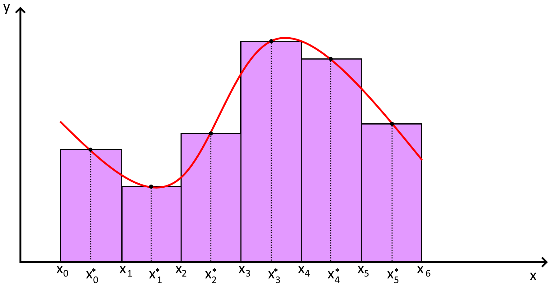
Assume that \(\{x_{0},x_{1},\ldots, x_{n}\}\) are \(n+1\) in \([a,b]\) such that

\[\begin{equation*} a=x_{0}<x_{1}<\cdots <x_{N-1}<x_{n}=b, \end{equation*}\]

and \(\Delta x_{j}\) is defined as \(\Delta x_{j}=x_{j+1}-x_{j}\). Then,

(5.51)\[\begin{equation}\label{NI_midpoint_eq01} \int_{{\,a}}^{{\,b}}{{f\left( x \right)\,dx}} \approx \sum_{j=0}^{n-1}f(x^*_j) \Delta x_j, %\notag \\ & = f(x^{*}_{0}) \Delta x_{0} +f(x^{*}_{1}) \Delta x_{1} + \ldots + f(x^{*}_{n-1}) \Delta x_{n-1} \end{equation}\]

where \(x_{j}^{*} = (x_{j} + x_{j+1})/2\), for \( 0 \leq j \leq n-1\) are the midpoint of the intervals.

In case these points are equally distanced. i.e. \(\Delta x_{n}= h>0\) for \(n\in \{0,1,\ldots,N\}\), the midpoins \(x_{j}^{*}\) will be in the following form

\[\begin{equation*} x_{0}^{*} = a + \frac{1}{2}h,~x_{1}^{*} = x_{1} + \frac{1}{2}h = a + \frac{3}{2}h, \ldots, ,~x_{n-1}^{*} = x_{n-1} + a + \frac{1}{2}h = \frac{(2n-1)}{2}h. \end{equation*}\]

and

(5.52)\[\begin{equation}\label{NI_midpoint_eq02} \int _{a}^{b}f(x)\,dx \approx h\sum _{j=1}^{n} f\left(a+\frac{(2j-1)}{2}h\right) = f\left(a + \frac{1}{2}h\right) + f\left(a + \frac{3}{2}h\right) + \ldots + f\left(a+ \frac{(2n-1)}{2}h\right) \end{equation}\]

Python Code

import numpy as np

def Midpoint(f, a, b, N):
    '''
    Parameters
    ----------
    f : function 
        DESCRIPTION. A function. Here we use lambda functions
    a : float
        DESCRIPTION. a is the left side of interval [a, b]
    b : float
        DESCRIPTION. b is the right side of interval [a, b]
    N : int
        DESCRIPTION. Number of xn points

    Returns
    -------
    S : float
        DESCRIPTION. Numerical Integration of f(x) on [a,b]
        through Midpoint rule

    '''
     
    # discretizing [a,b] into N subintervals
    x = np.linspace(a, b, N+1)
    # midpoints
    xmid=(x[0:N]+x[1:N+1])/2
    # discretizing function f on [a,b]
    fn = f(xmid)
    # the increment h
    h = (b - a)/N
    ### Trapezoidal rule
    M = h * np.sum(fn)
    return M

MATLAB Code

function [M] = Midpoint(f, a, b, N)
%{
Parameters
----------
f : function 
    DESCRIPTION. A function. Here we use lambda functions
a : float
    DESCRIPTION. a is the left side of interval [a, b]
b : float
    DESCRIPTION. b is the right side of interval [a, b]
N : int
    DESCRIPTION. Number of xn points

Returns
-------
T : float
    DESCRIPTION. Numerical Integration of f(x) on [a,b]
    through Trapezoidal rule

%}
% discretizing [a,b] into N subintervals
x = linspace(a, b, N+1);
% discretizing function f on [a,b]
% the increment \delta x
h = (b - a) / N;
xm=(x(1:(n-1))+x(2:n))./2;
fx = f(xm);
M = h*sum(fx);

Example: Use the Midpoint rule and compute \({\displaystyle\int_{0}^{1} x^2\, dx}\) when when

• a) \(N = 5\),

• b) \(N = 10\).

Solution:

a. \(n = 5\): discretizing \([0,~1]\) using \(h = \dfrac{1-0}{5} = 0.2\), we get the following set of points,

\[\begin{equation*} \left\{ 0,~0.2,~0.4,~0.6,~0.8,~1.0 \right\}, \end{equation*}\]

and the midpoints are:

\[\begin{equation*} \left\{ \frac{0 + 0.2}{2} = 0.1,~\frac{0.2 + 0.4}{2} = 0.3,~\frac{0.4 + 0.6}{2} = 0.5,~\frac{0.6 + 0.8}{2} = 0.7,\frac{0.8 + 1.0}{2} = 0.9 \right\}. \end{equation*}\]

\noindent Now, we have,

\[\begin{align*} \int _{a}^{b}f(x)\,dx & \approx h\sum _{j=1}^{5} f\left(a+\frac{(2j-1)}{2}h\right) \notag \\ & = h\left(f(0.1)+f(0.3)+f(0.5)+f(0.7)+f(0.9)\right) = 0.330 \end{align*}\]

a. b \(n = 10\): discretizing \([0,~1]\) using \(h = \dfrac{1-0}{10}=0.1\),

\[\begin{equation*} \left\{ 0,~0.1,~0.2,~0.3,~0.4,~0.5,~0.6,~0.7,~0.8,~0.9,~1.0 \right\} \end{equation*}\]

and the midpoints are:

\[\begin{equation*} \left\{ 0.05,~0.15,~0.25,~0.35,~0.45,~0.55,~0.65,~0.75,~0.85,~0.95 \right\}. \end{equation*}\]

Therefore,

\[\begin{align*} \int _{a}^{b}f(x)\,dx & \approx h\sum _{j=1}^{10} f\left(a+\frac{(2j-1)}{2}h\right) \notag \\ & = h\left(f(0.05)+f(0.15)+f(0.25)+\cdots + f(0.85) +f(0.95)\right) = 0.3325 \end{align*}\]

Example: Use the Midpoint rule and compute

\[\begin{align*} \int_{0}^{\pi/4} \cos^2(x)\, dx, \end{align*}\]

when

• a) \(N = 5\),

• b) \(N = 10\).

Solution:

a. \(n = 5\): discretizing \([0,~\pi/4]\) using \(h = \dfrac{\pi/4}{5} = \dfrac{\pi }{20}\), we get the following set of points,

\[\begin{equation*} \left\{ 0,~\frac{\pi }{20},~\frac{\pi }{10},~\frac{3\,\pi }{20},~\frac{\pi }{5},~\frac{\pi }{4} \right\}, \end{equation*}\]

and the midpoints are:

\[\begin{equation*} \left\{ \frac{\pi }{40},~\frac{3\,\pi }{40},~\frac{\pi }{8},~\frac{7\,\pi }{40},~\frac{9\,\pi }{40} \right\}. \end{equation*}\]

We have,

\[\begin{align*} \int _{a}^{b}f(x)\,dx & \approx h\sum _{j=1}^{5} f\left(a+\frac{(2j-1)}{2}h\right) \notag \\ & = h\left(f\left( \frac{\pi }{40}\right) +f\left(\frac{3\,\pi }{40} \right)+f\left(\frac{\pi }{8}\right)+f\left(\frac{7\,\pi }{40}\right) + f\left(\frac{9\,\pi }{40}\right)\right) \notag \\ & = 0.64063952. \end{align*}\]

b. \(n = 10\): Similarly,

\[\begin{equation*} h = \frac{b- a}{n} = \frac{\pi/4}{10} = \frac{\pi}{40}. \end{equation*}\]

Thus, \hlg{\(n = 10\)}. Now, discretizing \([0,~\pi/4]\) using \(h = \dfrac{\pi}{40}\),

\[\begin{equation*} \left\{ 0,~\frac{\pi }{40},~\frac{\pi }{20},~\frac{3\,\pi }{40},~\frac{\pi }{10},~\frac{\pi }{8},~\frac{3\,\pi }{20},~\frac{7\,\pi }{40},~\frac{\pi }{5},~\frac{9\,\pi }{40},~\frac{\pi }{4} \right\} \end{equation*}\]

and the midpoints are:

\[\begin{equation*} \left\{ \frac{\pi }{80},~\frac{3\,\pi }{80},~\frac{\pi }{16},~\frac{7\,\pi }{80},~\frac{9\,\pi }{80},~\frac{11\,\pi }{80},~\frac{13\,\pi }{80},~\frac{3\,\pi }{16},~\frac{17\,\pi }{80},~\frac{19\,\pi }{80} \right\}. \end{equation*}\]

We get,

\[\begin{align*} \int _{a}^{b}f(x)\,dx & \approx h\sum _{j=1}^{10} f\left(a+\frac{(2j-1)}{2}h\right) \notag \\ & = h\left(f\left(\frac{\pi }{80}\right) +f\left(~\frac{3\,\pi }{80}\right)+f\left(\frac{\pi }{16}\right)+\cdots + f\left(\frac{17\,\pi }{80}\right) + f\left(\frac{19\,\pi }{80}\right) \right) \notag \\ & = 0.64218483. \end{align*}\]

import sys
sys.path.insert(0,'..')
import hd_tools as hd

Loading BokehJS ...

def MidPointPlots(f, a, b, N, ax = False, CL = 'Tomato', EC = 'Blue'):
    if not ax:
        fig, ax = plt.subplots(nrows=1, ncols=1, figsize=(8, 6))
    x = np.linspace(a, b, N+1)
    y = f(x)

    X = np.linspace(a, b, (N**2)+1)
    Y = f(X)
    
    # midpoints
    xmid=(x[0:N]+x[1:N+1])/2
    
    _ = ax.plot(X,Y)
    for i in range(N):
        ax.fill([x[i], x[i], x[i+1], x[i+1]], [0, f(x[i]), f(x[i+1]), 0], facecolor = CL,
                edgecolor= EC,alpha=0.3, hatch='', linewidth=1.5)
    _ = ax.scatter(xmid, f(xmid), color= 'red', edgecolor = 'Black')
    _ = ax.set_xlim([min(x), max(x)])
    _ = ax.set_xticks(x)
    _ = ax.set_ylim([0, max(y)])
    ax1 = ax.twiny()
    _ = ax1.set_xlim(a, b)
    _ = ax1.set_xticks(xmid)
    _ = ax1.tick_params(axis='x', labelcolor= 'Blue', width=3)
    _ = ax1.set_xlabel('Midpoints', color='Blue')

import numpy as np
import matplotlib.pyplot as plt
from matplotlib.font_manager import FontProperties
from IPython.display import display, Latex
from hd_Numerical_Integration_Algorithms import Midpoint  

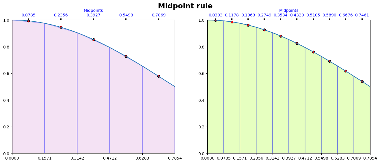
f = lambda x : np.cos(x)**2
a = 0
b = np.pi/4
N = [5, 10]
#
fig, ax = plt.subplots(nrows=1, ncols=len(N), figsize=(16, 6))
ax = ax.ravel()
Colors = ['Plum', 'GreenYellow']
font = FontProperties()
font.set_weight('bold')
_ = fig.suptitle("Midpoint rule", fontproperties=font, fontsize = 18)
for i in range(len(ax)):
    MidPointPlots(f= f, a = a, b= b, N = N[i], ax = ax[i], CL = Colors[i])
    Int_trapz = Midpoint(f= f, a = a, b= b, N = N[i])
    txt = 'h\sum _{j=1}^{%i} f\\left(a+j\\frac{h}{2}\\right) = %.4e'
    display(Latex(txt % (N[i], Int_trapz)))
    del Int_trapz
del i

\[h\sum _{j=1}^{5} f\left(a+j\frac{h}{2}\right) = 6.4373e-01\]

\[h\sum _{j=1}^{10} f\left(a+j\frac{h}{2}\right) = 6.4296e-01\]

5.4.1. Error Estimation

Theorem: Error Estimation for Midpoint rule

The error for the Midpoint rule is bounded (in absolute value) by

(5.53)\[\begin{equation}\label{Midpoint_Error_01} E_{h} = \left|\int _{a}^{b}f(x)\,dx - h\sum _{j=1}^{n} f\left(a+j\frac{h}{2}\right)\right| = \frac {(b-a)}{24}h^{2} \left|f''(\xi)\right|, \qquad \text{for some }\xi \in [a, b]. \end{equation}\]

for some \(\xi \in [a, b]\). Furthermore, if \(|f^{(2)}(x)|\leq M\)

(5.54)\[\begin{equation}\label{Midpoint_Error_02} E_{h} \leq M \,\frac {(b-a)^3}{24\,n^2} = M \,\frac {(b-a)}{24}h^{2}. \end{equation}\]

Proof:

The error for subinterval \([x_{i},~x_{i+1}]\) would be,

(5.55)\[\begin{align} \int_{x_i}^{x_{i+1}} f(x) dx -hf(c_i) &= \int_{x_i}^{x_{i+1}}(f(x)-f(c_i))dx \notag \\ & = \int_{x_i}^{x_{i+1}} \left(f(c_i)+f'(c_i)(x-c_i) + \frac{f''(\xi_i(x))}{2}(x-c_i)^2\;-\;f(c_i)\right) dx \notag \\ & = \frac{f''(\xi_i)}{2}\int_{x_i}^{x_{i+1}}(x-c_i)^2 dx = \frac{f''(\xi_i) h^3}{24} \end{align}\]

Note that in the above, we used the mean value theorem for integrals as \((x - c_{i})^2\) always outputs a positive value (sign does not change) that

(5.56)\[\begin{align} \int_{x_i}^{x_{i+1}} \frac{f''(\xi_i(x))}{2}(x-c_i)^2 dx = \frac{f''(\xi_i)}{2} \int_{x_i}^{x_{i+1}} (x-c_i)^2 dx \end{align}\]

Now, if you take the sum over the \(n\) intervals, we have,

(5.57)\[\begin{align} \sum_{i=1}^n \frac{f''(\xi_i) h^3}{24} = \frac{h^2(b-a)}{24}\left(\frac 1n \sum_{i=1}^n f''(\xi_i)\right) = \frac{h^2(b-a) f''(\xi)}{24}. \end{align}\]

For the above, note that since \(f\in C^2\), the term \(\frac 1n \sum f''(\xi_i)\) can be seen as an average of values of \(f''(\xi_i)\) and it is located in between the minimum and maximum of \(f''\). According to the intermediate value theorem, it will correspond to \(f''(\xi)\), for some \(\in(a,b)\).

Example: Assume that we want to use the Midpoint rule to approximate \({\displaystyle\int_{0}^{2} \frac{1}{1+x}\, dx}\). Find the smallest \(n\) for this estimation that produces an absolute error of less than \(5 \times 10^{-6}\). Then, evaluate \({\displaystyle\int_{0}^{2} \frac{1}{1+x}\, dx}\) using the Midpoint rule to verify the results.

Solution: We know that

\[\begin{align*} \int_{0}^{2} \frac{1}{1+x}\, dx = \ln(x+1) \Big|_{0}^{2} = \ln(3). \end{align*}\]

Also,

\[\begin{align*} f(x) = \frac{1}{x+1} & \quad \Rightarrow \quad f'(x) = -\frac{1}{(x + 1)^2} \quad \Rightarrow \quad f''(x) = \frac{2}{(x + 1)^3}. \end{align*}\]

From Example \ref{Ex.Trap.02}, we know also know that,

\[\begin{align*} M = \max_{0 \leq x \leq 2}|f''(x)| = 2. \end{align*}\]

It follows from solving the following inequality \eqref{Midpoint_Error_02} that

\[\begin{align*} \frac{(b -a)^3}{24\,n^2} M \leq 5\times 10^{-06} \quad \Rightarrow \quad & \frac{(2 - 0)^3}{24\,n^2}(2) < 5\times 10^{-6} \\ \quad \Rightarrow \quad & \frac{16}{24\,n^2} < 5\times 10^{-6}. \\ \quad \Rightarrow \quad & \frac{2}{3\,n^2} < 5\times 10^{-6}. \\ \quad \Rightarrow \quad & n^2 > \frac{2}{3(5\times 10^{-6})} = \frac{4}{1.5\times 10^{-5}} \\ \quad \Rightarrow \quad & n > \sqrt{\frac{4}{1.5\times 10^{-5}}} = 365.1483716701107 \end{align*}\]

To test this the above \(n\), let \(n = 366\) (the smallest integer after 365.1484). We have,

import numpy as np
E = 5e-6
# f'(x)
f = lambda x : 1/(x+1)
# f''(x)
f2 =  lambda x : 2/((x+1)**3)
Exact = np.log(3)
a =0; b= 2;
x = np.linspace(a, b)
M = max(abs(f2(x)))
N = int(np.ceil(np.sqrt((M*(b-a)**3)/(24* E))))
print('N = %i' %N)
# Trapezoidal rule
T = Midpoint(f, a, b, N)
Eh = abs(T - Exact)
print('Eh = %.4e' % Eh)

N = 366
Eh = 1.1059e-06

Example: For

\[\begin{equation*} \int_{0}^{2} \frac{1}{1 + x}\,dx = \ln(3), \end{equation*}\]

use Python/MATLAB show that the order of convergence for the Midpoint rule is indeed 2 numerically!

Solution:

import pandas as pd
a = 0; b = 2; f = lambda x : 1/(x+1); Exact = np.log(3)
N = [10*(2**i) for i in range(1, 10)]
Error_list = [];
for n in N:
    T = Midpoint(f = f, a = a, b = b, N = n)
    Error_list.append(abs(Exact - T))
Table = pd.DataFrame(data = {'h':[(b-a)/n for n in N], 'N':N, 'Eh': Error_list})
    
display(Table.style.set_properties(subset=['h', 'N'], **{'background-color': 'PaleGreen', 'color': 'Black',
       'border-color': 'DarkGreen'}).format(dict(zip(Table.columns.tolist()[-3:], 3*["{:.4e}"]))))

hd.derivative_ConvergenceOrder(vecs = [Table['Eh'].values], labels = ['Midpoint rule'], xlabel = r"$$i$$",
                               ylabel = " E_{h_{i}} / E_{h_{i-1}}",
                               title = 'Order of accuracy: Midpoint rule',
                               legend_orientation = 'horizontal')

	h	N	Eh
0	1.0000e-01	2.0000e+01	3.6965e-04
1	5.0000e-02	4.0000e+01	9.2548e-05
2	2.5000e-02	8.0000e+01	2.3145e-05
3	1.2500e-02	1.6000e+02	5.7869e-06
4	6.2500e-03	3.2000e+02	1.4467e-06
5	3.1250e-03	6.4000e+02	3.6169e-07
6	1.5625e-03	1.2800e+03	9.0422e-08
7	7.8125e-04	2.5600e+03	2.2606e-08
8	3.9063e-04	5.1200e+03	5.6514e-09