2.2. Fixed-point iteration

Definition

For a function \(g\), The point \(c\) is called a fixed point if

\[\begin{equation*} g(c) = c. \end{equation*}\]

For example \(c = 2\) is a fixed point for \(g(x) = x^2 -2\). As \(2 = g(2)\). To identify this point from \(g(x) = x^2 -2\), we can solve the following equation for \(c\)

\[\begin{equation*} c^2 -2 = c \quad \Rightarrow \quad c^2 -c - 2=0 \quad \Rightarrow \quad (c+1)(c-2) = 0 \quad \Rightarrow \quad \begin{cases} c = 2,\\ c = -1. \end{cases} \end{equation*}\]

Note that every point for function \(h(x) = x\) is a fixed point. Fixed point for function \(g(x) = x^2 - 2\) can be also seen as points that are on \(g(x)\) and \(h(x)\) at the same time (see the above Figure).

Theorem

a. If \(g\) is continuous on \([a, b]\) (i.e. \(g\in C[a, b]\)) and \(g(x) \in [a, b]\) for all values of \(x\) from \([a, b]\), then \(g\) has at least one fixed point in \([a, b]\).

b. In addition to part (a), if \(g'(x)\) exists on \((a, b)\) and a positive constant \(k < 1\) exists such that $\(|g'(x)| \leq k,\quad x\in (a,b),\)\( then there is a unique fixed point in \)[a, b]$.

Proof:

a. In case, \(g(a) = a\) or \(g(b) = b\), then \(g\) has a fixed point at one of the endpoints \(a\) or \(b\). If not, since \(g(x) \in [a, b]\), then \(g(a) > a\) and \(g(b) < b\). Since \(g\) is continuous on \([a, b]\), the function \(h(x) = g(x)-x\) is continuous on \([a, b]\). Also, \(h(a) = g(a) - a > 0\) and \(h(b) = g(b) - b < 0\).

Now, it follows from the Intermediate Value Theorem that there exists \(c \in (a, b)\) for which \(h(c) = 0\). Thus,

(2.7)\[\begin{equation} 0 = h( c) = g( c) - c \quad \Rightarrow \quad g( c) = c. \end{equation}\]

This number \(c\) is a fixed point for \(g\). b.
In addition to the assumptions from part (a), assume that \(|g'(x)| \leq k < 1\) and that \(c_{1}\) and \(c_{2}\) are both fixed points in \([a, b]\). If \(c_{1} \neq c_{2}\), then the Mean Value Theorem implies that a number \(\xi\) exists between \(c_{1}\) and \(c_{2}\), and hence in \([a, b]\), with

(2.8)\[\begin{equation}\label{eq2.8} g(c_{1}) - g(c_{2}) = \left(c_{1} - c_{2}\right) g'(\xi) \end{equation}\]

Since \(c_{1}\) and \(c_{2}\) are fixed points, then \(c_{1} = g(c_{1})\) and \(c_{2} = g(c_{2}\). It follows that,

(2.9)\[\begin{equation} | c_{1} - c_{2}| = |g(c_{1}) - g(c_{2}) = |g'(\xi)|| c_{1} - c_{2}| \leq k | c_{1} - c_{2}|. \end{equation}\]

Now, since \(|g'(x)| \leq k < 1\), we have,

(2.10)\[\begin{equation} | c_{1} - c_{2}| < | c_{1} - c_{2}|, \end{equation}\]

which is a contradiction. This contradiction must come from the assumption that there are two fixed points, \(c_{1} \neq c_{2}\). Hence, \(c_{1} = c_{2}\) and the fixed point in \([a, b]\) is unique.

Example: Show that

\[\begin{equation*} g(x)=\sqrt{x}. \end{equation*}\]

has a unique fixed point on the interval \([0.4, 1]\).

Solution:

The maximum and minimum values of \(g(x)\) for x in \([0.4, 1]\) must occur either when \(x\) is an endpoint of the interval or when the derivative is \(0\). Since \(g'(x) = \dfrac{1}{2\sqrt{x}}\), the function \(g\) is continuous and \(g'(x)\) exists on \([0.4, 1]\). Also,

\[\begin{equation*} g'(x) = 0 \quad \Rightarrow \quad \frac{1}{2\sqrt{x}} = 0 \quad \Rightarrow \quad \text{has no root in } (\infty, \infty). \end{equation*}\]

The maximum and minimum values of \(g(x)\) occur at \(x = 0.4\) or \(x = 1\). But \(g(0.4) = 0.63\) and \(g(1) = 1\). Therefore, the absolute maximum for \(g(x\)) on \([0.4, 1]\) occurs at \(x = 1\) and the absolute minimum \(g(x\)) on \([0.4, 1]\) occurs at \(x = 0.4\).

On the other hand, \(\dfrac{1}{2\sqrt{x}}\) is a decreasing function over \((0.4, 1)\) and

(2.11)\[\begin{equation}]\label{eq2.11} g'(x) = \left|\frac{1}{2\sqrt{x}}\right| \leq \frac{1}{2\sqrt{0.4}} = 0.79 < 1,\qquad x\in (0.4, 1). \end{equation}\]

Therefore, \(g\) satisfies all the hypotheses of the above theorem and has a unique fixed point in \([0, 1]\).

Note that here, \(k = 0.79\).

2.2.1. Fixed-Point Iteration

Approximating the fixed point of a function \(g\), we set an initial approximation \(c_{0}\) and produce the sequence \(\{c_n\}_{n=0}^{\infty}\) by setting \(c_{n} = g( c_{n-1})\) with \(n = 0,1,2,\ldots\). If the sequence converges to \(c\) and \(g\) is continuous, then

(2.12)\[\begin{equation} c = \lim_{n \to \infty} c_{n-1} = \lim_{n \to \infty} g(c_{n-1}) = g\left( \lim_{n \to \infty} c_{n-1}\right) = g(c), \end{equation}\]

is the approximation of solution to \(x = g(x)\) is obtained.

The following theorem is Theorem 2.4 from [Burden and Faires, 2005].

Theorem: Fixed-Point Theorem

If function \(g\) is continuous on \([a,b]\), and \(g(x) \in [a, b]\) for all \(x\) values from \([a, b]\). In addition, if \(g'(x)\) exists on \((a, b)\) and \(|g'(x)| \leq k\) for all \(x\) values from \([a, b]\) and some value of \(0<k<1\). Then, the sequence generated by \(c_n = g(c_{n-1})\) converges to a unique \textbf{fixed point} in \([a, b]\).

Proof: It follows from the previous theorem that a unique fixed-point \(c\) exists in \([a, b]\) with \(g(c) = c\). Since \(g(x) \in [a, b]\) for all \(x \in [a, b]\), the sequence \(\{ c_n\}_{n = 0}^{\infty}\) is defined for all \(n \geq 0\), and \(c_n \in [a, b]\) for \(n\geq 0\).

Now since \(|g'(x)| \leq k\), it follows from the \textbf{Mean Value Theorem} (Theorem \ref{MeanValueTheorem_theorem}) that

(2.13)\[\begin{equation} g(c_{n-1}) - g(c) = g'(\xi)(c_{n-1} - c) \end{equation}\]

Therefore,

(2.14)\[\begin{equation} |c_{n} - c| = |g(c_{n-1}) - g(c)| = |g'(\xi)| |c_{n-1} - c| \leq k |c_{n-1} - c| \end{equation}\]

where \(\xi_n \in (a, b)\). Applying this inequality inductively gives

(2.15)\[\begin{equation}\label{eq2.4} |c_{n} - c| \leq k |c_{n-1} - c| \leq k^{2} |c_{n-2} - c| \leq \dots \leq k^{n} |c_{0} - c|. \end{equation}\]

Since \(0<k<1\), we have

(2.16)\[\begin{equation} \lim_{n \to \infty} |c_{n} - c| \leq \lim_{n \to \infty} k^{n} |c_{0} - c| = 0. \end{equation}\]

Note that since \(k<1\)

\[\begin{equation*} \lim_{n \to \infty} k^{n} = 0. \end{equation*}\]

Therefore, \(\{ c_n\}_{n = 0}^{\infty}\) converges to \(c\).

The following theorem is Corollary 2.5 from [Burden and Faires, 2005].

Theorem

Assume that the hypotheses of Theorem \ref{Fixed_Point_th02} is in place, then bounds for the error involved in using sequence \(\{ c_n\}_{n = 0}^{\infty}\) to approximate \(c\) are given by

(2.17)\[\begin{equation} |c_{n} - c| \leq k^{n} \max\{c_0 - a, b - c_0\}, \end{equation}\]

and

(2.18)\[\begin{equation} |c_{n} - c| \leq \frac{k^{n}}{1 - k} |c_{1} - c_{0}|\quad n\geq 1. \end{equation}\]

Proof: As \(c \in [a,~b]\), we have,

(2.19)\[\begin{equation} |c_{n} - c| \leq k |c_{n-1} - c| \leq k^{n} \max \{c_{0} - a,~b-c_{0}\}. \end{equation}\]

Now, for \(n\geq 1\), it follows that,

(2.20)\[\begin{equation} |c_{n+1} - c_{n} | = |g( c_{n}) - g( c_{n-1}) | \leq k |c_{n} - c_{n-1}| \leq \dots \leq k^{n} |c_{1} - c_{0}|. \end{equation}\]

Therefore, for \(m> n \geq 1\), it follows that

(2.21)\[\begin{align} |c_{m} - c_{n} | &= |c_{m} - c_{m-1} + c_{m-1} + \dots - c_{n+1} + c_{n+1} - c_{n} | \notag \\ & \leq |c_{m} - c_{m-1}| + |c_{m-1} - c_{m-2}| + \dots + |c_{n+1} - c_{n}| \notag \\ & \leq k^{m-1} |c_{1} - c_{0}| + k^{m-2} |c_{1} - c_{0}| + \dots + k^{n} |c_{1} - c_{0}| \notag \\ & = k^{n} |c_{1} - c_{0}| (1 + k + k^2 + \dots + k^{m-n-1}) = k^{n} |c_{1} - c_{0}| \sum_{i = 0}^{m-n-1} k^{i}. \end{align}\]

On the other hand, \(\lim_{m \to \infty} c_{m} = c\); therefore,

(2.22)\[\begin{equation} |c - c_{n} | = \lim_{m \to \infty} |c_{m} - c_{n} | \leq \lim_{m \to \infty} k^{n} |c_{1} - c_{0}| \sum_{i = 0}^{m-n-1} k^{i} \leq k^{n} |c_{1} - c_{0}| \sum_{i = 0}^{\infty} k^{i}. \end{equation}\]

Observe that \(\sum_{i = 0}^{\infty} k^{i}\) is a geometric series with ratio \(k\) and \(0 < k < 1\). Thus,

(2.23)\[\begin{equation} |c - c_{n} | \leq \frac{k^{n}}{1 - k} |c_{1} - c_{0}|. \end{equation}\]

Assume that \(g(x)\) is a real function on a real values domain \([a,b]\). Then, given \(x_{0} \in [a,b]\), the fixed point iteration is

(2.24)\[\begin{equation} c_{n+1}=g(c_{n}),\quad n=0,1,2,\dots. \end{equation}\]

Python Code

import pandas as pd 
import numpy as np

def Fixed_Point(g, x0, TOL, Nmax):
    '''
    Parameters
    ----------
    g : function 
        DESCRIPTION. A function. Here we use lambda functions
    a : float
        DESCRIPTION. a is the left side of interval [a, b]
    b : float
        DESCRIPTION. b is the right side of interval [a, b]
    Nmax : Int, optional
        DESCRIPTION. Maximum number of iterations. The default is 1000.
    TOL : float, optional
        DESCRIPTION. Tolerance (epsilon). The default is 1e-4.

    Returns
    -------
    a dataframe
    '''
    
    xn = np.zeros(Nmax, dtype=float)
    En = np.zeros(Nmax, dtype=float)
    xn[0] = x0
    En[0] = x0
    
    for n in range(0, Nmax-1):
        xn[n+1] = g(xn[n])
        En[n+1] = np.abs(xn[n+1]-xn[n])
        if En[n+1] < TOL:
            return pd.DataFrame({'xn': xn[0:n+2], 'En': En[0:n+2]})
    return None

MATLAB Code

function [xn, En] = Fixed_Point(g, x0, TOL, Nmax)
%{
Parameters
----------
g : function 
    DESCRIPTION. A function. Here we use lambda functions
a : float
    DESCRIPTION. a is the left side of interval (a, b)
b : float
    DESCRIPTION. b is the right side of interval (a, b)
Nmax : Int, optional
    DESCRIPTION. Maximum number of iterations. The default is 1000.
TOL : float, optional
    DESCRIPTION. Tolerance (epsilon). The default is 1e-4.

Returns
-------
xn, En

Example: g = @(x) sqrt(x)
%}

switch nargin
    case 3
        Nmax = 1000;
    case 2
        TOL = 1e-4; Nmax = 1000;
end

xn = zeros(Nmax, 1);
En = zeros(Nmax, 1);

% initial values
xn(1) = x0;
En(1) = x0;

for n = 1:(Nmax-1)
    xn(n+1) = g(xn(n));
    En(n+1) = abs(xn(n+1)-xn(n));
    if En(n+1) < TOL
        xn = xn(1:n+1);
        En = En(1:n+1);
        return
    end
end

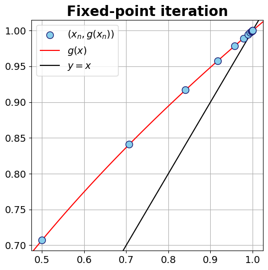
Example: Find a root of the following polynomial.

We know that

\[\begin{equation*} g(x)=\sqrt{x}. \end{equation*}\]

has a unique fixed point on the interval \([0.4, 1]\). Find a root of \(f(x)=x - \sqrt{x}\) on the interval \([0.4, 1]\) using the fixed point, \(g(x)\) and \(c_0 = 0.5\).

Solution: First, we need to convert \(f(x) = 0\) into the form \(x = g(x)\). That is

Since \(g(x)=\sqrt{x}\) has a unique fixed point on the interval \([0.4, 1]\), then

\[\begin{equation*} f(x) = x - \sqrt{x} = x - g(x) = 0 \end{equation*}\]

has a root on the interval \([0.4, 1]\). Thus, the fixed point of \(g\) is a root for \(f\). We can generate the entries of series \(\{c_{0}, c_{1}, c_{2}, \ldots\}\) using \(c_{n} = g(c_{n-1})\) and \(c_{0} = 0.5\). We have,

\[\begin{equation*} \begin{array}{lcl} c_{0} = 0.5 & \Rightarrow & c_{1} = g(c_{0}) = g(0.5) = 0.707107 \\ c_{1} = 0.707107 & \Rightarrow & c_{2} = g(c_{1}) = g(0.707107) = 0.840896 \\ c_{2} = 0.840896 & \Rightarrow & c_{3} = g(c_{2}) = g(0.840896) = 0.917004 \\ c_{3} = 0.917004 & \Rightarrow & c_{4} = g(c_{3}) = g(0.917004) = 0.957603 \\ \vdots & \vdots & \vdots \end{array} \end{equation*}\]

We reproduce a sequence \(\{c_{0}, c_{1}, c_{2}, \ldots\}\) using \(g(x)\) in a way that converges to the fixed point if \(n\) is large enough. Then, \(f(x)\) will converge to the root for when \(n\) is large enough. In doing so, we can use our python script to generale \(\{c_{0}, c_{1}, c_{2}, \ldots\}\).

# This part is used for producing tables and figures
import sys
sys.path.insert(0,'..')

import hd_tools as hd
import numpy as np
g = lambda x : np.sqrt(x)
from hd_RootFinding_Algorithms import Fixed_Point
data = Fixed_Point(g = g, x0 = .5, TOL=1e-4, Nmax=20)
display(data.style.format({'En': "{:.4e}"}))

Loading BokehJS ...

	xn	En
0	0.500000	1.0000e+00
1	0.707107	2.0711e-01
2	0.840896	1.3379e-01
3	0.917004	7.6108e-02
4	0.957603	4.0599e-02
5	0.978572	2.0969e-02
6	0.989228	1.0656e-02
7	0.994599	5.3714e-03
8	0.997296	2.6966e-03
9	0.998647	1.3511e-03
10	0.999323	6.7621e-04
11	0.999662	3.3828e-04
12	0.999831	1.6918e-04
13	0.999915	8.4602e-05

Note that here \(E_n =|c_{n} - c_{n-1}|\) and we stopped the iterations when \(E_n < 10^{-4}\). Here, \(E_{0}\) was set to 1 since the previous step is not available.

import matplotlib.pyplot as plt

fontsize = 14
Fig_Params = ['legend.fontsize','axes.labelsize','axes.titlesize','xtick.labelsize','ytick.labelsize']
Fig_Params = dict(zip(Fig_Params, len(Fig_Params)*[fontsize]))
plt.rcParams.update(Fig_Params)
    
fig, ax = plt.subplots(1, 1, figsize=(6, 6))
_ = ax.scatter(data.xn, g(data.xn), s= 100, facecolors='SkyBlue',
               edgecolors='MidnightBlue', label = r'$(x_{n}, g(x_{n}))$', zorder = 3)
xlim = ax.get_xlim()
ylim = ax.get_ylim()
x = np.linspace(xlim[0], xlim[1])
y = g(x)
_ = ax.plot(x, g(x), 'r', label = r'$g(x)$')
_ = ax.plot(x, x, 'k', label = r'$y = x$')
_ = ax.legend()
_ = ax.set_xlim(xlim)
_ = ax.set_ylim(ylim)
_ = ax.yaxis.grid()
_ = ax.xaxis.grid(True, which='major')
_ = ax.set_title('Fixed-point iteration', fontsize = 20, weight = 'bold')

Example:

a. Show that \(g(x) = \sqrt[3]{x + 2}\) has a unique fixed point on \([0, 2]\).

b. Assuming that \(c_{0} = 0\), estimate the number of iterations required to achieve \(10^{-4}\) accuracy.

c. Use fixed-point iteration to find an approximation to the fixed point that is accurate to within \(10^{-4}\) (here the exact fixed-point is \(c = c = 1.5213797068045676\)).

Solution:

a. We have,

\[\begin{equation*} g(x) = \sqrt[3]{x + 2} \quad \Rightarrow \quad g'(x) = \frac{1}{3 (2 + x)^{2/3}}, \end{equation*}\]

\(g\) is continuous and \(g'\) exists on \([0, 2]\). Thus, \(g\) has at least one fixed point in \([a, b]\).

Since \(\dfrac{1}{3 (2 + x)^{2/3}}\) is a decreasing function, then \(g'(x)\) gets its maximum value at \(x = 0\), and

\[\begin{equation*} |g'(x)| = \frac{1}{3 (2 + x)^{2/3}} \leq \frac{1}{3 (2 + 0)^{2/3}} = \frac{1}{3 (2)^{2/3}} = 0.21 < 1, \quad x \in [0, 2]. \end{equation*}\]

\textbf{Fixed Point theorem} implies that there a unique fixed point \(c\) exists in \([0, 2]\).

Note that we can see that \(k = 0.21 = \dfrac{1}{5}\).

b. Note that from part (a), \(k = 0.21\), and with \(c_{0} = 0\), we have \(c_{1} = 1.2599\). Moreover,

\[\begin{equation*} |c_{n} - c| \leq \frac{k^{n}}{1-k} |c_{1} - c_{0}| = \frac{(0.21)^n}{1-0.21}(1.2599)=\left( 0.21 \right)^{n} \left(1.25\right) \left( 1.2599 \right) = 1.5749\left( 0.21 \right)^{n} \end{equation*}\]

Also,

\[\begin{align*} 1.5749 \left( 0.21 \right)^{n} \leq 10^{-4} & \quad \Rightarrow \quad \left( 0.21 \right)^{n} \leq \frac{0.0001}{1.5749} = 6.3496 \times 10^{-5} \\ & \quad \Rightarrow \quad \ln \left( 0.21\right)^{n} \leq \ln \left( 6.3496 \times 10^{-5}\right) \\ & \quad \Rightarrow \quad n\, \left( -1.56)\right) \leq \ln \left( 6.3496 \times 10^{-5}\right) = -9.6645 \end{align*}\]

It follows that,

\[\begin{equation*} -1.56\, n \leq -9.6645 \quad \Rightarrow \quad 1.56n \geq 9.6645 \quad \Rightarrow \quad n \geq \frac{9.6645}{1.56} \approx 6.2 \end{equation*}\]

The above computations shows, we need at least 7 iterations to ensure an accuracy of \(10^{-4}\). c. We have,

g = lambda x : (x + 2)**(1/3)
data = Fixed_Point(g = g, x0 = .5, TOL=1e-4, Nmax=20)
display(data.style.format({'En': "{:.4e}"}))

	xn	En
0	0.500000	1.0000e+00
1	1.357209	8.5721e-01
2	1.497360	1.4015e-01
3	1.517913	2.0553e-02
4	1.520880	2.9676e-03
5	1.521308	4.2754e-04
6	1.521369	6.1575e-05

fig, ax = plt.subplots(1, 1, figsize=(6, 6))
_ = ax.scatter(data.xn, g(data.xn), s= 100, facecolors='SkyBlue',
               edgecolors='MidnightBlue', label = r'$(x_{n}, g(x_{n}))$', zorder = 3)
xlim = ax.get_xlim()
ylim = ax.get_ylim()
x = np.linspace(xlim[0], xlim[1])
y = g(x)
_ = ax.plot(x, g(x), 'r', label = r'$g(x)$')
_ = ax.plot(x, x, 'k', label = r'$y = x$')
_ = ax.legend()
_ = ax.set_xlim(xlim)
_ = ax.set_ylim(ylim)
_ = ax.yaxis.grid()
_ = ax.xaxis.grid(True, which='major')
_ = ax.set_title('Fixed-point iteration', fontsize = 20, weight = 'bold')

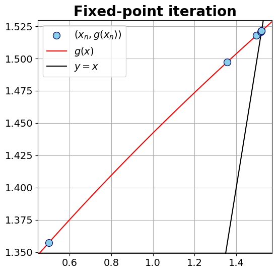
Note that here \(E_n =|c_{n} - c_{n-1}|\) and we stopped the iterations when \(n = N_{\max} = 7\), and \(E_{0}\) was set to 1 since the previous step is not available. Since, \(c = 1.5213797068045676\), we have,

\[\begin{equation*} \text{Absolute Error for } c_{7} = | 1.5213773037708966 - 1.5213797068045676| = 2.403034\times 10^{-06}. \end{equation*}\]