2.3. Newton methods#
2.3.1. Newton’s method#
Assume that \(f \in C^2[a, b]\) and let \(c_0\) be a point in \([a,b]\) such that
approximate root \(c\) for \(f\)
\(c_0\) it is not a root of \(f\) (i.e. \(f(c_0) \neq 0\))
\(|c - c_0|\) is very small!
Then, using Taylor expansion, we have,
where \(\xi(c)\) lies between \(c\) and \(c_0\). Since \(f(c) = 0\) and \(|c - c_0|\) is a very small number, then \((c - c_0)^2\) is even smaller number. Therefore,
\noindent \begin{minipage}[t]{0.49\textwidth} \vfill It follows from solving the above equation for \(c\) that,
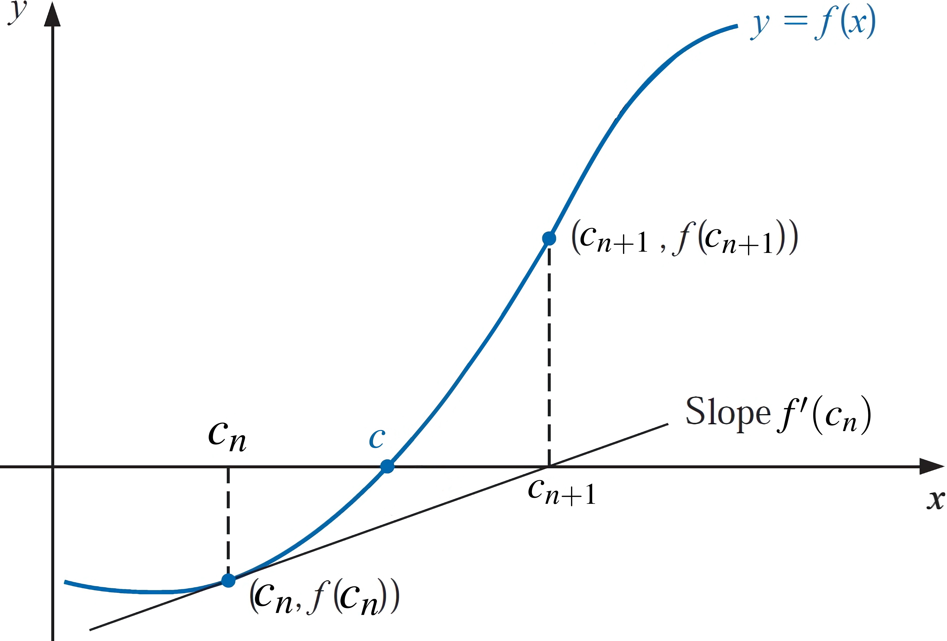
Fig. 2.1 Newton’s method. The approximation \(c_{n+1}\) is the x-intercept of the tangent line to the graph of \(f\) at \((c_{n}, f(c_{n}))\).#
Now, let \(c_1\) denote \(c_0 - f(c_0)/f'(c_0)\). Then, a sequence of approximations \(\{ c_n\}_{n = 0}^{\infty}\) can be generated through intimal approximation \(c_{0}\) as follows,
The Newton-Raphson method is a root-finding algorithm that iteratively approximates the roots of a real-valued function. A single-variable function \(f\), its derivative \(f'\), and an initial guess \(c_{0}\) for a root of \(f\) are required for this method. The procedure is repeated iteratively as follows:
The following proposition is Exercise 29 from 1.1 of [Burden and Faires, 2005].
Theorem
a. Suppose \(f (c) = 0\). Then, there exists a real number \(\delta > 0\) with \(f (x) = 0\), for all \linebreak\(x \in [c - \delta, c + \delta]\), with \([c - \delta, c + \delta] \subseteq [a, b]\).
b. Suppose \(f (c) = 0\) and \(k > 0\) is given. Then, there exists a real number \(\delta > 0\) such that \(|f (x)| \leq k\) for all \(x \in [c - \delta, c + \delta]\), with \([c - \delta, c + \delta] \subseteq [a, b]\).
The following theorem is Theorem 2.6 from [Burden and Faires, 2005].
Theorem: Convergence using Newton’s Method
Assume that \(f \in C^2[a, b]\) and let \(c\) be a point in \([a,b]\) such that \(f(c) = 0\) while \(f'(c) \neq 0\). Then, there is a positive value such as \(\delta > 0\) such that, for \textbf{any} initial approximation \(c_0 \in [c - \delta, c + \delta]\), Newton’s method induces a sequence \(\{ c_n\}_{n = 0}^{\infty}\) converging to \(c\).
Proof: Let
where
Now assume that \(k\) is a real number in \((0, 1)\). First, let’s find an interval \([c - \delta, c + \delta]\) that \(g\) maps into itself and for which
Observe that \(f'\) is continuous and \(f'( c) \neq 0\), then there is a \(\delta_{1}>0\) exists such that \(f'(x) \neq 0\) for \(x \in [c - \delta_{1}, c + \delta_{1}]\subseteq [a,b]\). Therefore, \(g\) is defined and continuous on \([c - \delta_{1}, c + \delta_{1}]\). Now, since
Since \(f \in C^2[a, b]\), we have \(g \in C^{1}[c - \delta_{1}, c + \delta_{1}]\).
On the other hand, since \(f ( c) = 0\), it follows that,
Since \(g'\) is continuous and \(0 < k < 1\), there exists a \(\delta\), with \(0 < \delta < \delta_1\), and
Next we demonstrate that \(g\) maps \([c - \delta, c + \delta]\) into itself. In case, \(x \in [c - \delta, c + \delta]\), the \textbf{Mean Value Theorem} implies that for some number \(\xi\) between \(x\) and \(c\),
Therefore,
Because \(x \in [c - \delta, c + \delta]\), it follows that \(|x - c| < \delta\) and that \(|g(x) - c| < \delta\). Thus, \(g\) maps \([c - \delta, c + \delta]\) into itself.
All the hypotheses of the \textbf{Fixed-Point Theorem} are now satisfied, so the sequence \(\{ c_n\}_{n = 0}^{\infty}\) defined by
converges to \(c\) for any \(c_0 \in [c - \delta, c + \delta]\).
import pandas as pd
import numpy as np

def Newton_method(f, Df, x0, TOL = 1e-4, Nmax = 100, Frame = True):
    '''
    Parameters
    ----------
    f : function
        DESCRIPTION.
    Df : function
        DESCRIPTION. the derivative of f
    x0 : float
        DESCRIPTION. Initial estimate
    TOL : TYPE, optional
        DESCRIPTION. Tolerance (epsilon). The default is 1e-4.
    Nmax : Int, optional
        DESCRIPTION. Maximum number of iterations. The default is 100.
    Frame : bool, optional
        DESCRIPTION. If it is true, a dataframe will be returned. The default is True.

    Returns
    -------
    xn, fxn, Dfxn, n
    or
    a dataframe

    '''

    xn=np.zeros(Nmax, dtype=float)
    fxn=np.zeros(Nmax, dtype=float)
    Dfxn=np.zeros(Nmax, dtype=float)
    xn[0] = x0
    for n in range(0,Nmax-1):
        fxn[n] = f(xn[n])
        if abs(fxn[n]) < TOL:
            Dfxn[n] = Df(xn[n])
            if Frame:
                return pd.DataFrame({'xn': xn[:n+1], 'fxn': fxn[:n+1], 'Dfxn': Dfxn[:n+1]})
            else:
                return xn, fxn, Dfxn, n
        Dfxn[n] = Df(xn[n])
        if Dfxn[n] == 0:
            print('Zero derivative. No solution found.')
            return None
        xn[n+1] = xn[n] - fxn[n]/Dfxn[n]
    print('Exceeded maximum iterations. No solution found.')
    return None
function [xn, fxn, Dfxn, n] = Newton_method(f, Df, x0, TOL, Nmax)
%{
Parameters
----------
f : function
    DESCRIPTION.
Df : function
    DESCRIPTION. the derivative of f
x0 : float
    DESCRIPTION. Initial estimate
TOL : TYPE, optional
    DESCRIPTION. Tolerance (epsilon). The default is 1e-4.
Nmax : Int, optional
    DESCRIPTION. Maximum number of iterations. The default is 100.

Returns
-------
xn, fxn, Dfxn, n
or
a dataframe

Example
f = @(x) x^3 - x - 2
Df = @(x) 3*x^2-1
%}

switch nargin
    case 4
        Nmax = 100;
    case 3
        TOL = 1e-4; Nmax = 100;
end


xn = zeros(Nmax, 1);
fxn = zeros(Nmax, 1);
Dfxn = zeros(Nmax, 1);
xn(1) = x0;
for n = 1:(Nmax-1)
    fxn(n) = f(xn(n));
    if abs(fxn(n)) < TOL
        Dfxn(n) = Df(xn(n));
        xn = xn(1:n+1);
        fxn = fxn(1:n+1);
        Dfxn = Dfxn(1:n+1);
        return
    end
    Dfxn(n) = Df(xn(n));
    if Dfxn(n) == 0
        disp('Zero derivative. No solution found.')
        xn = xn(1:n+1);
        fxn = fxn(1:n+1);
        Dfxn = Dfxn(1:n+1);
        return
    end
    xn(n+1) = xn(n) - fxn(n)/Dfxn(n);
end
disp('Exceeded maximum iterations. No solution found.')
Example:
\(f(x)=x^{3}-x-2\) has the following real root
a. Show that Newton’s method can generate a sequence \(\{ c_n\}_{n = 0}^{\infty}\) converging to \(c\). b. Approximate a root of \(f(x)=x^{3}-x-2\) using Newton’s method on \([1,~2]\) with \(c_{0} = 1\).
Solution: a. Since \(f(x)=x^{3}-x-2\) is a polynomial, then \(f \in C^2[1,~2]\). Also, using the following figure, we can see that \(f(x)\) has a root around point \(c\).
On the other hand, \(f'(x)=3x^2-1\). Thus, we can see that, with \(c=1.5213797068045676\),
Thus, according to the \textbf{Convergence using Newton’s Method}, there is a positive value such as \(\delta > 0\) such that, for \textbf{any} initial approximation \(c_0 \in [1 - \delta, 2 + \delta]\), Newton’s method induces a sequence \(\{ c_n\}_{n = 0}^{\infty}\) converging to \(c\). b. To identify a few entries of the sequence \(\{ c_n\}_{n = 0}^{\infty}\), we need both \(f(x)\) and \(f'(x)\) for Newton’s method. Thus,
Then,
We can use our python script to generate \(\{c_{0}, c_{1}, c_{2}, \ldots\}\).
# This part is used for producing tables and figures
import sys
sys.path.insert(0,'..')
import hd_tools as hd


from hd_RootFinding_Algorithms import Newton_method

f = lambda x: x**3 - x - 2
Df = lambda x: 3*x**2-1

data = Newton_method(f, Df, x0 = 1, TOL = 1e-4, Nmax = 20)
display(data.style.format({'fxn': "{:.4e}"}))
hd.it_method_plot(data, title = 'Newton Method', ycol = 'fxn', ylabel = 'f(xn)')
2.3.2. The Secant Method#
Observe that in Newton’s method, \(f'(c_{n})\) can be approximated as follows
Thus,
This also can be simplified as follows
Remark
Herein, we call the sequence generated by \eqref{Secant_Method_eq} the Secant method, and the one produced by \eqref{simplified_Secant_Method_eq} as the simplified Secant method. For the following example, we only use the Secant method \eqref{Secant_Method_eq}, and applying the simplified Secant method \eqref{simplified_Secant_Method_eq} will be left as an exercise.
import pandas as pd
import numpy as np

def Secant_method(f, x0, x1, TOL = 1e-4, Nmax = 100, Frame = True):
    '''
    Parameters
    ----------
    f : function
        DESCRIPTION.
    x0 : float
        DESCRIPTION. First initial estimate
    x1 : float
        DESCRIPTION. Second initial estimate
    TOL : TYPE, optional
        DESCRIPTION. Tolerance (epsilon). The default is 1e-4.
    Nmax : Int, optional
        DESCRIPTION. Maximum number of iterations. The default is 100.
    Frame : bool, optional
        DESCRIPTION. If it is true, a dataframe will be returned. The default is True.

    Returns
    -------
    xn, fxn, Dfxn, n
    or
    a dataframe

    '''

    xn=np.zeros(Nmax, dtype=float)
    fxn=np.zeros(Nmax, dtype=float)

    xn[0] = x0
    xn[1] = x1
    for n in range(1, Nmax-1):
        fxn[n] = f(xn[n])
        if abs(fxn[n]) < TOL:
            if Frame:
                return pd.DataFrame({'xn': xn[:n+1], 'fxn': fxn[:n+1]})
            else:
                return xn, fxn, n
        Dfxn = (f(xn[n]) - f(xn[n-1])) / (xn[n] - xn[n-1])
        if Dfxn == 0:
            print('Zero derivative. No solution found.')
            return None
        xn[n+1] = xn[n] - fxn[n]/Dfxn
    print('Exceeded maximum iterations. No solution found.')
    return None
function [xn, fxn, Dfxn, n] = Secant_method(f, x0, x1, TOL, Nmax)
%{
Parameters
----------
f : function
    DESCRIPTION.
x0 : float
    DESCRIPTION. First initial estimate
x1 : float
    DESCRIPTION. Second initial estimate
TOL : TYPE, optional
    DESCRIPTION. Tolerance (epsilon). The default is 1e-4.
Nmax : Int, optional
    DESCRIPTION. Maximum number of iterations. The default is 100.

Returns
-------
xn, fxn, Dfxn, n
or
a dataframe

Example
f = @(x) x^3 - x - 2
%}

switch nargin
    case 4
        Nmax = 100;
    case 3
        TOL = 1e-4; Nmax = 100;
end


xn = zeros(Nmax, 1);
fxn = zeros(Nmax, 1);
xn(1) = x0;
xn(2) = x1;
for n = 2:(Nmax-1)
    fxn(n) = f(xn(n));
    if abs(fxn(n)) < TOL
        xn = xn(1:n+1);
        fxn = fxn(1:n+1);
        return
    end
    Dfxn = (f(xn(n)) - f(xn(n-1))) / (xn(n) - xn(n-1));
    if Dfxn == 0
        disp('Zero derivative. No solution found.')
        xn = xn(1:n+1);
        fxn = fxn(1:n+1);
        return
    end
    xn(n+1) = xn(n) - fxn(n)/Dfxn;
end
disp('Exceeded maximum iterations. No solution found.')
Example: Use the Secant method for finding the root of the function from the previous Example.
Solution:
We have,
Then, using \(c_0 = 1\) and \(c_{1} = 1.2\), we have,
We can use our python script to generate \(\{c_{0}, c_{1}, c_{2}, \ldots\}\).
from hd_RootFinding_Algorithms import Secant_method

f = lambda x: x**3 - x - 2

data = Secant_method(f, x0 = 1, x1 = 1.2, TOL = 1e-4, Nmax = 20)
display(data.style.format({'fxn': "{:.4e}"}))
hd.it_method_plot(data, title = 'Secant Method', ycol = 'fxn', ylabel = 'f(xn)')
| xn | fxn | |
|---|---|---|
| 0 | 1.000000 | 0.0000e+00 |
| 1 | 1.200000 | -1.4720e+00 |
| 2 | 1.757576 | 1.6717e+00 |
| 3 | 1.461078 | -3.4204e-01 |
| 4 | 1.511439 | -5.8633e-02 |
| 5 | 1.521858 | 2.8462e-03 |
| 6 | 1.521376 | -2.1830e-05 |
Remark
We also could identify \(c_{1}\) using the Newton method and then continue with the Secant method for \(n\geq 2\).
2.3.3. The Method of False Position (Regula Falsi)#
The method of False Position (also called Regula Falsi) induces estimations in a similar way to the Secant method, but with a subtle change. This change is a test to assure that the root is bracketed between subsequent iterations.
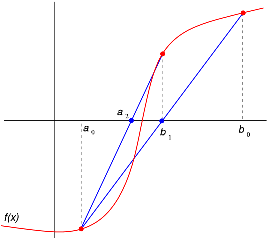
Fig. 2.2 The first two iterations of the second method. The red curve represents the function \(f\) and the blue lines are the secants corresponding to \(a_{1}\) and \(a_{2}\). The image source with slight modifications: https://en.wikipedia.org/wiki/Regula_falsi#
In this method, the root of the equation \(f(x) = 0\) for the real variable \(x\) is estimated when \(f\) is a continuous function defined on a closed interval \([a, b]\) and where \(f(a)\) and \(f(b)\) have opposite signs. Moreover, \(c_n\) is identified:
def Regula_falsi(f, a, b, Nmax = 1000, TOL = 1e-4, Frame = True):
    '''
    Parameters
    ----------
    f : function
        DESCRIPTION. A function. Here we use lambda functions
    a : float
        DESCRIPTION. a is the left side of interval [a, b]
    b : float
        DESCRIPTION. b is the right side of interval [a, b]
    TOL : float, optional
        DESCRIPTION. Tolerance (epsilon). The default is 1e-4.
    Frame : bool, optional
        DESCRIPTION. If it is true, a dataframe will be returned. The default is True.

    Returns
    -------
    an, bn, cn, fcn, n
    or
    a dataframe
    '''

    if f(a)*f(b) >= 0:
        print("Regula falsi method is inapplicable .")
        return None

    # let c_n be a point in (a_n, b_n)
    an=np.zeros(Nmax, dtype=float)
    bn=np.zeros(Nmax, dtype=float)
    cn=np.zeros(Nmax, dtype=float)
    fcn=np.zeros(Nmax, dtype=float)
    # initial values
    an[0]=a
    bn[0]=b

    for n in range(0,Nmax-1):
        cn[n]= (an[n]*f(bn[n]) - bn[n]*f(an[n])) / (f(bn[n]) - f(an[n]))
        fcn[n]=f(cn[n])
        if f(an[n])*fcn[n] < 0:
            an[n+1]=an[n]
            bn[n+1]=cn[n]
        elif f(bn[n])*fcn[n] < 0:
            an[n+1]=cn[n]
            bn[n+1]=bn[n]
        else:
            print("Regula falsi method fails.")
            return None
        if (abs(fcn[n]) < TOL):
            if Frame:
                return pd.DataFrame({'an': an[:n+1], 'bn': bn[:n+1], 'cn': cn[:n+1], 'fcn': fcn[:n+1]})
            else:
                return an, bn, cn, fcn, n

    if Frame:
        return pd.DataFrame({'an': an[:n+1], 'bn': bn[:n+1], 'cn': cn[:n+1], 'fcn': fcn[:n+1]})
    else:
        return an, bn, cn, fcn, n
function [an, bn, cn, fcn, n] = Regula_falsi(f, a, b, Nmax, TOL)
%{
Parameters
----------
f : function
    DESCRIPTION. A function. Here we use lambda functions
a : float
    DESCRIPTION. a is the left side of interval [a, b]
b : float
    DESCRIPTION. b is the right side of interval [a, b]
Nmax : Int, optional
    DESCRIPTION. Maximum number of iterations. The default is 1000.
TOL : float, optional
    DESCRIPTION. Tolerance (epsilon). The default is 1e-4.

Returns
-------
an, bn, cn, fcn, n
or
a dataframe

Example: f = @(x) x^3 - x - 2
%}
if nargin==4
    TOL= 1e-4;
end

if f(a)*f(b) >= 0
    disp("Regula falsi is inapplicable .")
    return
end

% let c_n be a point in (a_n, b_n)
an = zeros(Nmax, 1);
bn = zeros(Nmax, 1);
cn = zeros(Nmax, 1);
fcn = zeros(Nmax, 1);
% initial values
an(1) = a;
bn(1) = b;

for n = 1:(Nmax-1)
    cn(n)= (an(n)*f(bn(n)) - bn(n)*f(an(n))) / (f(bn(n)) - f(an(n)));
    fcn(n)=f(cn(n));
    if f(an(n))*fcn(n) < 0
        an(n+1)=an(n);
        bn(n+1)=cn(n);
    elseif f(bn(n))*fcn(n) < 0
        an(n+1)=cn(n);
        bn(n+1)=bn(n);
    else
        disp("Regula falsi method fails.")
    end
    if (abs(fcn(n)) < TOL)
        return
    end
end
Example: Use the Method of False Position for finding the root of the function from the previous Example.
Solution:
we have,
Then, let \(a_{0} = 1\) and \(b_{0} = 2\), then
Now, since \hlg{\(f(a_0)f(c_0) < 0\)} and \(f(c_0)f(b_0) > 0\), we set \(a_{1} = a_{0}\) and \(b_{1} = c_{0}\). Then,
Then, since \hlg{\(f(a_1)f(c_1) < 0\)} and \(f(c_1)f(b_1) > 0\), we set \(a_{2} = c_{1}\) and \(b_{2} = b_{1}\).
In addition, using the python script, we have,
from hd_RootFinding_Algorithms import Regula_falsi
a=1; b=2;
data = Regula_falsi(f, a, b, Nmax = 20, TOL = 1e-4)
display(data.style.format({'fcn': "{:.4e}"}))
hd.it_method_plot(data, title = 'Regula falsi')
hd.root_plot(f, a, b, [data.an.values[:-1], data.an.values[-1]], ['an', 'root'])
| an | bn | cn | fcn | |
|---|---|---|---|---|
| 0 | 1.000000 | 2.000000 | 1.333333 | -9.6296e-01 |
| 1 | 1.333333 | 2.000000 | 1.462687 | -3.3334e-01 |
| 2 | 1.462687 | 2.000000 | 1.504019 | -1.0182e-01 |
| 3 | 1.504019 | 2.000000 | 1.516331 | -2.9895e-02 |
| 4 | 1.516331 | 2.000000 | 1.519919 | -8.6751e-03 |
| 5 | 1.519919 | 2.000000 | 1.520957 | -2.5088e-03 |
| 6 | 1.520957 | 2.000000 | 1.521258 | -7.2482e-04 |
| 7 | 1.521258 | 2.000000 | 1.521344 | -2.0935e-04 |
| 8 | 1.521344 | 2.000000 | 1.521370 | -6.0461e-05 |
2.3.4. Regula Falsi (The Illinois algorithm)#
There have been also some improved versions of Regula Falsi. For example, in the Illinois algorithm, \(c_n\) is estimated as follows.
def Regula_falsi_Illinois_alg(f, a, b, Nmax = 1000, TOL = 1e-4, Frame = True):
    '''
    Parameters
    ----------
    f : function
        DESCRIPTION. A function. Here we use lambda functions
    a : float
        DESCRIPTION. a is the left side of interval [a, b]
    b : float
        DESCRIPTION. b is the right side of interval [a, b]
    TOL : float, optional
        DESCRIPTION. Tolerance (epsilon). The default is 1e-4.
    Frame : bool, optional
        DESCRIPTION. If it is true, a dataframe will be returned. The default is True.

    Returns
    -------
    an, bn, cn, fcn, n
    or
    a dataframe
    '''

    if f(a)*f(b) >= 0:
        print("Regula falsi (Illinois algorithm) method is inapplicable .")
        return None

    # let c_n be a point in (a_n, b_n)
    an=np.zeros(Nmax, dtype=float)
    bn=np.zeros(Nmax, dtype=float)
    cn=np.zeros(Nmax, dtype=float)
    fcn=np.zeros(Nmax, dtype=float)
    # initial values
    an[0]=a
    bn[0]=b

    for n in range(0,Nmax-1):
        cn[n]= (0.5*an[n]*f(bn[n]) - bn[n]*f(an[n])) / (0.5*f(bn[n]) - f(an[n]))
        fcn[n]=f(cn[n])
        if f(an[n])*fcn[n] < 0:
            an[n+1]=an[n]
            bn[n+1]=cn[n]
        elif f(bn[n])*fcn[n] < 0:
            an[n+1]=cn[n]
            bn[n+1]=bn[n]
        else:
            print("Regula falsi (Illinois algorithm) method fails.")
            return None
        if (abs(fcn[n]) < TOL):
            if Frame:
                return pd.DataFrame({'an': an[:n+1], 'bn': bn[:n+1], 'cn': cn[:n+1], 'fcn': fcn[:n+1]})
            else:
                return an, bn, cn, fcn, n

    if Frame:
        return pd.DataFrame({'an': an[:n+1], 'bn': bn[:n+1], 'cn': cn[:n+1], 'fcn': fcn[:n+1]})
    else:
        return an, bn, cn, fcn, n
function [an, bn, cn, fcn, n] = Regula_falsi_Illinois_alg(f, a, b, Nmax, TOL)
%{
Parameters
----------
f : function
    DESCRIPTION. A function. Here we use lambda functions
a : float
    DESCRIPTION. a is the left side of interval [a, b]
b : float
    DESCRIPTION. b is the right side of interval [a, b]
Nmax : Int, optional
    DESCRIPTION. Maximum number of iterations. The default is 1000.
TOL : float, optional
    DESCRIPTION. Tolerance (epsilon). The default is 1e-4.

Returns
-------
an, bn, cn, fcn, n
or
a dataframe

Example: f = @(x) x^3 - x - 2
%}
if nargin==4
    TOL= 1e-4;
end

if f(a)*f(b) >= 0
    disp("Regula falsi (Illinois algorithm) method is inapplicable .")
    return
end

% let c_n be a point in (a_n, b_n)
an = zeros(Nmax, 1);
bn = zeros(Nmax, 1);
cn = zeros(Nmax, 1);
fcn = zeros(Nmax, 1);
% initial values
an(1) = a;
bn(1) = b;

for n = 1:(Nmax-1)
    cn(n)= (0.5*an(n)*f(bn(n)) - bn(n)*f(an(n))) / (0.5*f(bn(n)) - f(an(n)));
    fcn(n)=f(cn(n));
    if f(an(n))*fcn(n) < 0
        an(n+1)=an(n);
        bn(n+1)=cn(n);
    elseif f(bn(n))*fcn(n) < 0
        an(n+1)=cn(n);
        bn(n+1)=bn(n);
    else
        disp("Regula falsi (Illinois algorithm) method fails.")
    end
    if (abs(fcn(n)) < TOL)
        return
    end
end
from hd_RootFinding_Algorithms import Regula_falsi_Illinois_alg
data = Regula_falsi_Illinois_alg(f, a, b, Nmax = 20, TOL = 1e-4)
display(data.style.format({'fcn': "{:.4e}"}))
hd.it_method_plot(data, title = 'Regula falsi (Illinois algorithm)', color = 'Purple')
hd.root_plot(f, a, b, [data.an.values[:-1], data.an.values[-1]], ['an', 'root'])
| an | bn | cn | fcn | |
|---|---|---|---|---|
| 0 | 1.000000 | 2.000000 | 1.500000 | -1.2500e-01 |
| 1 | 1.500000 | 2.000000 | 1.529412 | 4.8036e-02 |
| 2 | 1.500000 | 1.529412 | 1.524671 | 1.9614e-02 |
| 3 | 1.500000 | 1.524671 | 1.522877 | 8.9069e-03 |
| 4 | 1.500000 | 1.522877 | 1.522090 | 4.2212e-03 |
| 5 | 1.500000 | 1.522090 | 1.521723 | 2.0394e-03 |
| 6 | 1.500000 | 1.521723 | 1.521547 | 9.9423e-04 |
| 7 | 1.500000 | 1.521547 | 1.521462 | 4.8682e-04 |
| 8 | 1.500000 | 1.521462 | 1.521420 | 2.3888e-04 |
| 9 | 1.500000 | 1.521420 | 1.521399 | 1.1734e-04 |
| 10 | 1.500000 | 1.521399 | 1.521389 | 5.7666e-05 |