5.1. Introduction#
Antiderivative of the function
A function \(F\) is called an \textbf{antiderivative} of the function \(f\) on an interval \([a,~b]\) if [Strang, Herman, and others, 2016]
for all \(x\in [a,~b]\).
Let \(F\) denote an antiderivative of \(f\) on an interval \([a,~b]\), then the most \textbf{general antiderivative of \(f\)} on \([a,~b]\) is \(F(x)+C\) where \(C\) is an arbitrary constant [Strang, Herman, and others, 2016]. This indicates that if \(f\) has an antiderivative \(F\), there are an infinite number of antiderivatives for \(f\) that may be formed by adding an arbitrary constant to \(F\).
Example: For example,
a. \(F_{1}(x) = -\cos(x) + C\) is the general antiderivative for \(f_{1}(x) = \sin(x)\),
b. \(F_{2}(x) = \dfrac{x^{n+1}}{n+1} + C\) is the general antiderivative for \(f_{2}(x) = x^{n}\) with \(n\neq -1\).
The link between differentiation and integration is established by the Fundamental Theorem of Calculus, Part 1 [Strang, Herman, and others, 2016].
Fundamental Theorem of Calculus, Part 1
Let \(f(x)\) be a continuous function over \([a,~b]\), and the function \(F(x\)) can defined by \cite{strang2016calculus}
then \(F'(x)=f(x)\) on \([a,~b]\).
Proof: It follows from the definition of the derivative that,
Observe that \eqref{FTC.eq02} is simnply the average of the function \(f(x)\) on \([x,~x+h]\). Thus, by the Mean Value Theorem for Integrals (Theorem \ref{MVT_Int}), there exists a number \(c\) in \([x,~x+h]\) such that \cite{strang2016calculus}
Furthermore, since \(c \in [x,~x+h]\), \(c\) approaches \(x\) as \(h\) gets closer to zero. Moreover, since \(f(x)\) is a continuous function, we have
Combining all of these elements, we have
Fundamental Theorem of Calculus, Part 2
Let \(f(x)\) be a continuous function over \([a,~b]\), \(F(x)\) any antiderivative of \(f(x)\) then [Strang, Herman, and others, 2016]
Proof: Define \(P = \{x_{i} \}\) with \(i = 0,1,\ldots,n\) as a a partition of \([a,~b]\). Then, we have,
Now, since \(F(x)\) is an antiderivative of \(f(x)\) on \([a,~b]\), by the Mean Value Theorem (Theorem \ref{MeanValueTheorem_theorem}), there are points \(c_{i} \in [x_{i-1},~x_{i}]\) with \(i = 1,2,\ldots,n\) such that,
It follows from \eqref{FTC.eq07} and \eqref{FTC.eq08} that
Finally, pushing \(n\to \infty\)
Typically, when we approximate an integral, we are doing so because it is difficult (or sometimes, it is not possible) to determine the exact value of the integral. Before, we expand on the numerical integration recall that,
Sigma Notation
Given the summation \(a_{0} + a_{1} + \ldots + a_{n}\), we express the sum in the compact form using sigma notation.
where \(\Sigma\) is the Greek letter sigma, which is employed as the summation symbol.
Remark
Note that \(\sum_{j = 0}^{n}a_{j}\) is read ‘’the sum as \(j\) goes from 0 to \(n\) of \(a_j\)``. However, this can be also expressed as follows,
Consider the following figure in which region \(S\) is bounded by the graph of a continuous function \(f\) [where \(f\geq 0\)], the vertical lines \(x= a\) and \(x= b\), and the x-axis. We like to determine the area of the region \(S\) that is beneath the curve \(y = (x)\) between \(a\) and \(b\). Calculating this area explicitly is not always straightforward or possible. We can estimate this area using a summation of the area of rectangles instead.
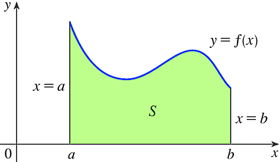
Fig. 5.1 \(S=s(x, y)~|~a\leq x\leq b,~0\leq y \leq ƒ(x)\).#
A quadrature rule is a numerical estimate of a function’s definite integral, commonly expressed as a weighted sum of function values at defined locations within the domain of integration. For \(i = 1,\ldots, n\), nodes \(x_i\) and weights \(w_i\) can be used to create an \(n\)-point quadrature rule.
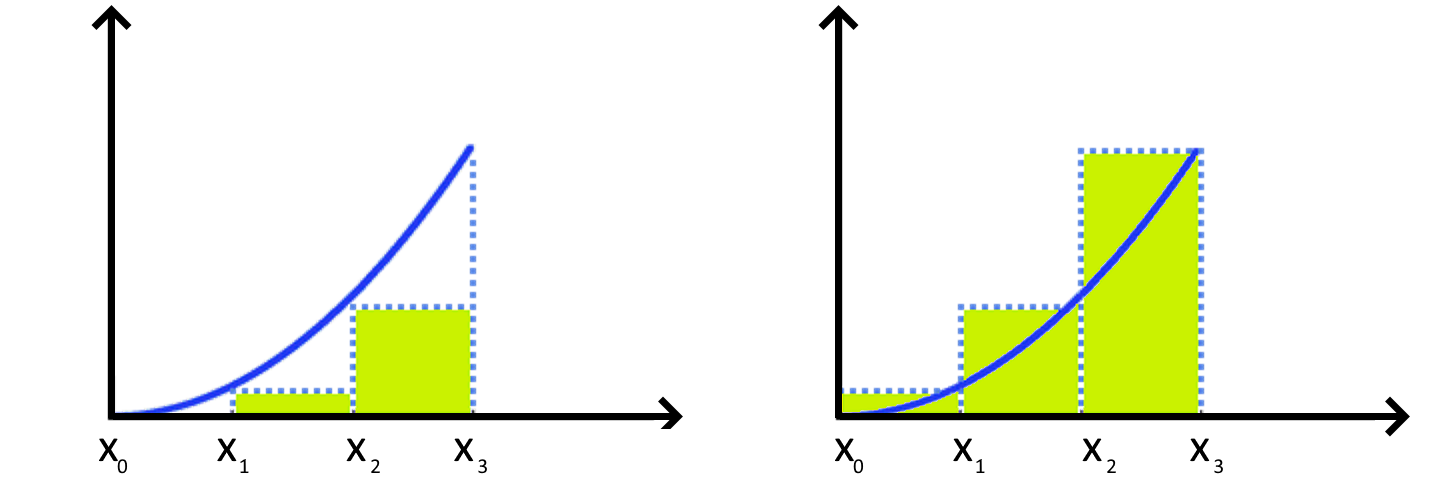
Fig. 5.2 Left-hand approximation of area using three subdivisions. \textbf{Right}: Right-hand approximation of area using three subdivisions.#
The left- and right-hand rule approaches from Riemann summations are the most straightforward ways for numerically approximating integrals. Assume that \(\{x_{0},~x_{1},\ldots,~x_{n}\}\) are \(n+1\) in \([a,b]\) such that
and \(\Delta x_{j}\) is defined as \(\Delta x_{j}=x_{j+1}-x_{j}\) with \(0 \leq j \leq n-1\). Then,
is a Riemann summation of \(f(x)\) on \([a,b]\) where \(c_j \in[x_{j},~x_{j+1}]\).
In case \(\{x_{0},x_{1},\ldots, x_{n}\}\) are equally distanced. i.e. \(\Delta x_{j}= h = \dfrac{b-a}{n}>0\) for \(j\in \{0,1,\ldots,n-1\}\),
import numpy as np

def LeftRiemannSum(f, a, b, N):
    '''
    Parameters
    ----------
    f : function
        DESCRIPTION. A function. Here we use lambda functions
    a : float
        DESCRIPTION. a is the left side of interval [a, b]
    b : float
        DESCRIPTION. b is the right side of interval [a, b]
    N : int
        DESCRIPTION. Number of xn points

    Returns
    -------
    L : float
        DESCRIPTION. Numerical Integration of f(x) on [a,b]
        through left Riemann sum rule

    '''

    # discretizing [a,b] into N subintervals
    # N must be an even integer

    # the increment h
    h = (b-a)/N
    # discretizing [a,b] into N subintervals
    x = np.linspace(a, b, N+1)

    fn = f(x)
    L = h * np.sum(fn[0:-1])
    return L
function [L] = LeftRiemannSum(f, a, b, N)
%{
Parameters
----------
f : function
    DESCRIPTION. A function. Here we use lambda functions
a : float
    DESCRIPTION. a is the left side of interval [a, b]
b : float
    DESCRIPTION. b is the right side of interval [a, b]
N : int
    DESCRIPTION. Number of xn points

Returns
-------
L : float
    DESCRIPTION. Numerical Integration of f(x) on [a,b]
    through left Riemann sum rule

%}
% discretizing [a,b] into N subintervals
x = linspace(a, b, N+1);
% discretizing function f on [a,b]
fn = f(x);
% the increment \delta x
h = (b - a) / N;
% Trapezoidal rule
L = h * sum(fn(1:N));
import numpy as np

def RightRiemannSum(f, a, b, N):
    '''
    Parameters
    ----------
    f : function
        DESCRIPTION. A function. Here we use lambda functions
    a : float
        DESCRIPTION. a is the left side of interval [a, b]
    b : float
        DESCRIPTION. b is the right side of interval [a, b]
    N : int
        DESCRIPTION. Number of xn points

    Returns
    -------
    L : float
        DESCRIPTION. Numerical Integration of f(x) on [a,b]
        through right Riemann sum rule

    '''

    # discretizing [a,b] into N subintervals
    # N must be an even integer

    # the increment h
    h = (b-a)/N
    # discretizing [a,b] into N subintervals
    x = np.linspace(a, b, N+1)

    fn = f(x)
    R = h * np.sum(fn[1:])
    return R
function [R] = RightRiemannSum(f, a, b, N)
%{
Parameters
----------
f : function
    DESCRIPTION. A function. Here we use lambda functions
a : float
    DESCRIPTION. a is the left side of interval [a, b]
b : float
    DESCRIPTION. b is the right side of interval [a, b]
N : int
    DESCRIPTION. Number of xn points

Returns
-------
L : float
    DESCRIPTION. Numerical Integration of f(x) on [a,b]
    through right Riemann sum rule

%}
% discretizing [a,b] into N subintervals
x = linspace(a, b, N+1);
% discretizing function f on [a,b]
fn = f(x);
% the increment \delta x
h = (b - a) / N;
% Trapezoidal rule
R = h * sum(fn(2:(N+1)));
Example: Approximate
with \(n = 10\) using the left- and right-hand rule approaches from Riemann summations. For each approximation, calculate the absolute error.
Solution:
Here \(n = 10\), and it follows from discretizing \([0,~2]\) using \(h = \dfrac{b-a}{n} = \dfrac{2-0}{10} = 0.2\) that
Left-hand rule summation:
Right-hand rule summation:
On the other hand, analytically, this can be calculated easily:
\noindent\hlr{Left-hand rule summation (absolute error):} \(E_{h} = |6 - 5.040000| = 0.960000\). \ \noindent\hlr{Right-hand rule summation (absolute error):} \(E_{h} = |6 - 7.040000| = 1.040000\).
Theorem
Let \(L_{n}\) and \(R_{n}\) show the left- and right-hand rule approaches from Riemann summations, respectively. Then,
Moreover, let \(f(x)\) be a differentiable function on \([a,~b]\) with \(f'(x)\) continuous \([a,~b]\), then,
where \(M_{1} = \max_{a\leq x \leq b} |f'(x)|\).
Proof: This proof is based on proof of a similar theorem from [Grinshpan, 2022]. Assume that \(f(x)\) is a bounded function on a bounded interval \([a,~b]\) and also assume that
are distinct points \([a,~b]\) that generate \(n\) subintervals \([x_{k-1},~x_{k}]\) where \(k = 1, 2, 3,\ldots , n\). Now, let \(x_{k}^{*}\) be a arbitrary point in \([x_{k-1},~x_{k}]\). Then, the error of \(k\)-th rectangle can be defined as follows,
Hence,
Now, it follows from adding these error bounds over \(k\),
Now, if \(h= x_{k} - x_{k-1}\) for \(k = 1, 2, 3,\ldots , n\), it follows that (why!?),
Example: For
use Python/MATLAB show that the order of convergence for the left- and right-hand rule approaches from Riemann summations are indeed 1 numerically!
Solution:
import sys
sys.path.insert(0,'..')
import hd_tools as hd

from hd_Numerical_Integration_Algorithms import LeftRiemannSum, RightRiemannSum
import numpy as np
import pandas as pd
N = [10*(2**i) for i in range(1, 10)]
a = 0; b = 2; f = lambda x : 1/(x+1); Exact = np.log(3);
LError_list = []; RError_list = []
for n in N:
    L = LeftRiemannSum(f = f, a = a, b = b, N = n)
    LError_list.append(abs(Exact - L))
    R = RightRiemannSum(f = f, a = a, b = b, N = n)
    RError_list.append(abs(Exact - R))
# DataFrame
Table = pd.DataFrame(data = {'h':[(b-a)/n for n in N], 'n':N,
                            'Eh (Left Reimann Sum)': LError_list,
                            'Eh (Right Reimann Sum)': RError_list})
display(Table)
| h | n | Eh (Left Reimann Sum) | Eh (Right Reimann Sum) | |
|---|---|---|---|---|
| 0 | 0.100000 | 20 | 0.034073 | 0.032593 |
| 1 | 0.050000 | 40 | 0.016852 | 0.016482 |
| 2 | 0.025000 | 80 | 0.008380 | 0.008287 |
| 3 | 0.012500 | 160 | 0.004178 | 0.004155 |
| 4 | 0.006250 | 320 | 0.002086 | 0.002080 |
| 5 | 0.003125 | 640 | 0.001042 | 0.001041 |
| 6 | 0.001563 | 1280 | 0.000521 | 0.000521 |
| 7 | 0.000781 | 2560 | 0.000260 | 0.000260 |
| 8 | 0.000391 | 5120 | 0.000130 | 0.000130 |
hd.derivative_ConvergenceOrder(vecs = [Table['Eh (Left Reimann Sum)'].values,
                                    Table['Eh (Right Reimann Sum)'].values],
                               labels = ['Left Reimann Sum', 'Right Reimann Sum'],
                               title = 'Order of accuracy: Left and Right Reimann Sums',
                               legend_orientation = 'horizontal', ylim = [0.9, 1.1])