6. Initial-Value Problems for Ordinary Differential Equations#
In this chapter, we go through several methods that can approximate the solution of a (well-posed) initial-value problem (IVP) on grid points.
A first order differential equation (ODE) is expressed as follows,
If \(y(a) = y_{0}\) is known, then the following ODE equation is an IVP:
Definition
In case function \(f(t,y)\) when \(t\) is a independent variable and \(y\) is a dependent variable defined on a domain \(D\subset \mathbb{R}^{2}\) and
then it is said that \(f\) satisfies the Lipschitz condition in the variable \(y\), and \(L\) is known as the Lipschitz constant.
Definition
Domain \(D\subset \mathbb{R}^{2}\) is called convex if any two points of this domain can be connected using a line while all points on this line stay in the Domain. In other words, for any two points \((t_{1}, y_{1}), (t_{2}, y_{2}) \in D\)
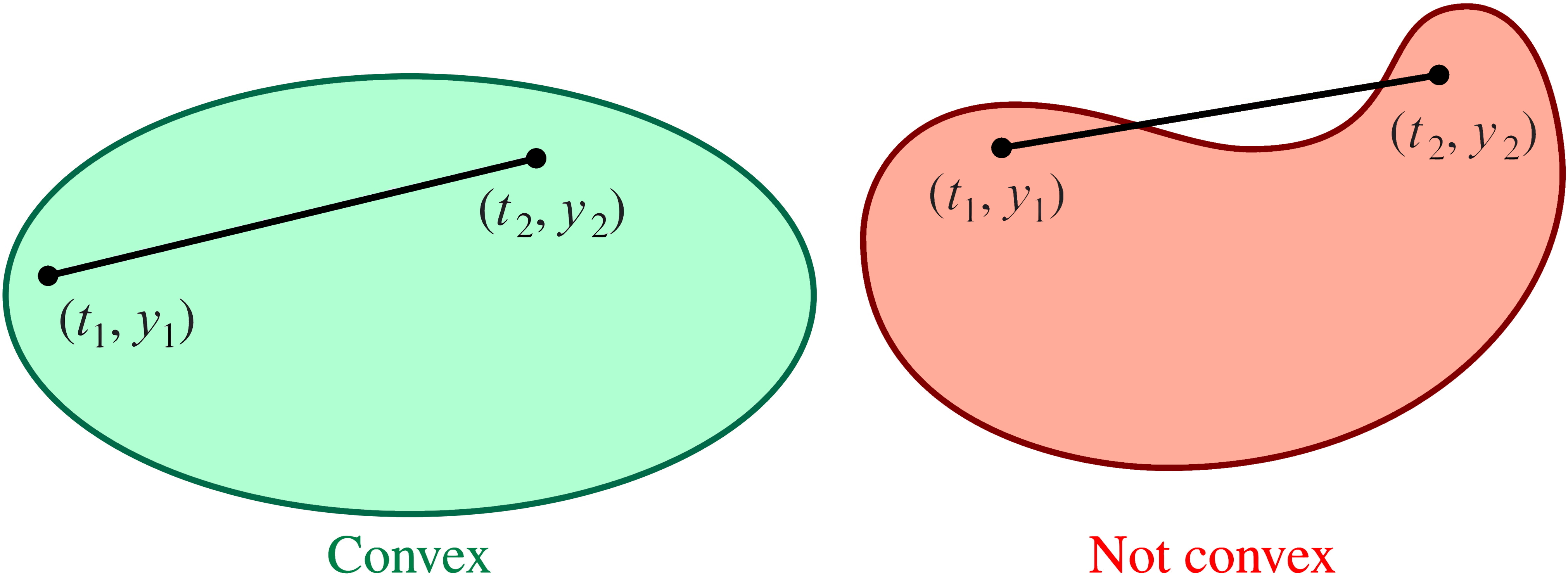
Fig. 6.2 An example of convex (left) and not convex (right) domain.#
Theorem
Assume that \(D\subset \mathbb{R}^{2}\) is a convex set and \(f(t,y)\) is defined on this set. If a constant \(L>0\) exists such that
then \(f\) satisfies the Lipschitz condition in the variable \(y\) and \(L\) is the Lipschitz constant.
Theorem
Assume that domain \(D = \{ (t, y):~a\leq t \leq b,~\infty<y \infty\}\) and \(f\in C(D)\). If \(f\) satisfies a Lipschitz condition on \(D\) in the variable \(y\), then the IVP,
has a unique solution \(y(t)\) when \(\leq t \leq b\).
Definition
The IVP $\(\begin{aligned} \frac{dy}{dt} &= f(t,y),& a \leq t \leq b,~y(a) = y_{0}, \end{aligned}\)$ is said to be a well-posed problem if
it has a solution and this solution is unique,
constants \(\varepsilon_{0} >0\) and \(k>0\) exists such that for any arbitrary value of \(\varepsilon > 0\) with \(\varepsilon_{0} > \varepsilon > 0\), whenever \(\delta(t)\) is continuous with \(|\delta(t)|<\varepsilon\) for all values of \(t \in [a,b]\), and when the IVP
\[\begin{align*} \frac{dy}{dt} &= f(t,z) + \delta(t),& a \leq t \leq b,~z(a) = y_{0} + \delta_{0}, \end{align*}\]has a unique solution \(z(t)\) that satisfies
\[\begin{align*} |z(t) - y(t) | < k \varepsilon, \quad t \in[a,b] \end{align*}\]
Remark
Roughly speaking, an IVP is said to be a well-posed problem if it has a unique solution whose value varies only negligibly if initial conditions change by a small value.