LDL decomposition

7.4. LDL decomposition#

LDL decomposition is very similar to Cholesky factorization; however, there are some subtle differences. In this decomposition, a (real) symmetric positive definite matrix $A$ is decomposed as follows

\begin{array}{r} A = L D L^{*}, \end{array}

where $L$ is a lower triangular matrix, and $D$ is a diagonal matrix.

Furthermore, We have,

\begin{array}{r} [\begin{array}{c} a_{11} & a_{12} & \dots & a_{1 n} \\ a_{21} & a_{22} & \dots & a_{2 n} \\ ⋮ & ⋮ & ⋮ \\ a_{n 1} & a_{n 2} & \dots & a_{n n} \end{array}] = [\begin{array}{c} 1 & 0 & \dots & 0 \\ l_{21} & 1 & \dots & 0 \\ ⋮ & ⋮ & ⋮ \\ l_{n 1} & l_{n 2} & \dots & 1 \end{array}] [\begin{array}{c} d_{11} & 0 & \dots & 0 \\ 0 & d_{22} & \dots & 0 \\ ⋮ & ⋮ & ⋮ \\ 0 & 0 & \dots & d_{n n} \end{array}] . \end{array}

Solving this system, $l_{i j}$ and $d_{i i}$ can be identified as follows

\begin{aligned} d_{i i} & = a_{i i} - \sum_{k = 1}^{i - 1} l_{i j}^{2} d_{j j}, \\ l_{i i} & = \frac{1}{d_{i i}} (a_{i j} - \sum_{k = 1}^{i - 1} l_{i k} l_{j k} d_{k k}), \end{aligned}

See [Allaire, Kaber, Trabelsi, and Allaire, 2008] for the full derivation of this algorithm.

Python Code

import numpy as np
import pandas as pd

def myLDL(A):
    '''
    Assuming that the matrix A is symmetric and positive definite,
    this function computes a unit lower triangular matrix L, and
    a diagonal matrix D, such that A = LDL^t
    Parameters
    ----------
    A : numpy array
        DESCRIPTION. Matrix A

    Returns
    -------
    L : numpy array
        DESCRIPTION. Matrix L from A = LDL^t
    D : numpy array
        DESCRIPTION. Matrix L from A = LDL^t

    '''
    
    n = A.shape[0]
    U = np.zeros([n,n], dtype = float)
    U[0, 0] = A[0, 0]
    U[1:, 0] = A[1:, 0]/U[0, 0]
    for j in range(1, n):
        U[j, j] = A[j, j]
        for k in range(0, j):
            U[j, j] = U[j, j] - U[k, k]*U[j, k]*U[j, k]
        for i in range(j+1, n):
            U[i, j] = A[i, j]
            for k in range(0, j):
                U[i, j] = U[i, j]- U[k, k]*U[i, k]*U[j, k]
            U[i, j] = U[i, j]/U[j, j]
    L = np.tril(U,-1) + np.eye(n, dtype=float)
    D = np.diag(np.diag(U))
    return L, D

MATLAB Code

function [L, D] = myLDL(A)
%{
Assuming that the matrix A is symmetric and positive definite,
this function computes a unit lower triangular matrix L, and
a diagonal matrix D, such that A = LDL^t
Parameters
----------
L : numpy array
    DESCRIPTION. Matrix L from A = LDL^t
D : numpy array
    DESCRIPTION. Matrix L from A = LDL^t
%}
n=length(A);
U = zeros(n,n);
U(1,1)=A(1,1);
U(2:n,1)=A(2:n,1)/U(1,1);
for j=2:n
   U(j,j)= A(j,j);
   for k=1:j-1
       U(j,j)=U(j,j)-U(k,k)*U(j,k)*U(j,k);
   end
   for i=j+1:n
       U(i,j)=A(i,j);
       for k=1:j-1
           U(i,j)=U(i,j)-U(k,k)*U(i,k)*U(j,k);
       end
       U(i,j)=U(i,j)/U(j,j);
   end
%
end
L = tril(U,-1)+eye(n,n);
D = diag(diag(U));

import sys
sys.path.insert(0,'..')
import hd_tools as hd

BokehJS 2.4.3 successfully loaded.

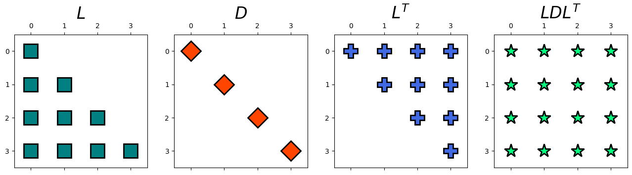
Example: Apply LDL decomposition on the following matrix and identify $L$ , $D$ , and $L$ .

\begin{array}{r} A = [\begin{array}{cccc} 7 & 3 & - 1 & 2 \\ 3 & 8 & 1 & - 4 \\ - 1 & 1 & 4 & - 1 \\ 2 & - 4 & - 1 & 6 \end{array}] . \end{array}

Solution: We have,

import numpy as np
from hd_Matrix_Decomposition import myLDL
from IPython.display import display, Latex
from sympy import init_session, init_printing, Matrix

A = np.array([ [7, 3, -1, 2], [3, 8, 1, -4], [-1, 1, 4, -1], [2, -4, -1, 6] ])
L, D = myLDL(A)
display(Latex(r'L ='), Matrix(np.round(L, 2)))
display(Latex(r'D ='), Matrix(np.round(D, 2)))
display(Latex(r'LD L^T ='), Matrix(np.round(np.matmul(L,np.matmul(D,L.T)), 2)))

L =

\begin{array}{r} [\begin{array}{c} 1.0 & 0 & 0 & 0 \\ 0.43 & 1.0 & 0 & 0 \\ - 0.14 & 0.21 & 1.0 & 0 \\ 0.29 & - 0.72 & 0.09 & 1.0 \end{array}] \end{array}

D =

\begin{array}{r} [\begin{array}{c} 7.0 & 0 & 0 & 0 \\ 0 & 6.71 & 0 & 0 \\ 0 & 0 & 3.55 & 0 \\ 0 & 0 & 0 & 1.89 \end{array}] \end{array}

L D L^{T} =

\begin{array}{r} [\begin{array}{c} 7.0 & 3.0 & - 1.0 & 2.0 \\ 3.0 & 8.0 & 1.0 & - 4.0 \\ - 1.0 & 1.0 & 4.0 & - 1.0 \\ 2.0 & - 4.0 & - 1.0 & 6.0 \end{array}] \end{array}

hd.matrix_decomp_fig(mats = [L, D, L.T, np.round(np.matmul(L,np.matmul(D,L.T)), 2)],
                     labels = ['$L$', '$D$','$L^T$', '$LD L^T$'], nrows=1, ncols=4, figsize=(16, 6))

../_images/83ef6893c9f156a523b7acb69554dd9c8212c7e184bd4f5c5fbf244f91853b71.png

Note that we could get a similar results using function, scipy.linalg.ldl.

import scipy.linalg as linalg
L, D, P = linalg.ldl(A)
display(Latex(r'L ='), Matrix(np.round(L, 2)))
display(Latex(r'D ='), Matrix(np.round(D, 2)))

L =

\begin{array}{r} [\begin{array}{c} 1.0 & 0 & 0 & 0 \\ 0.43 & 1.0 & 0 & 0 \\ - 0.14 & 0.21 & 1.0 & 0 \\ 0.29 & - 0.72 & 0.09 & 1.0 \end{array}] \end{array}

D =

\begin{array}{r} [\begin{array}{c} 7.0 & 0 & 0 & 0 \\ 0 & 6.71 & 0 & 0 \\ 0 & 0 & 3.55 & 0 \\ 0 & 0 & 0 & 1.89 \end{array}] \end{array}

7.4.1. Solving Linear systems using LDL decomposition#

We can solve the linear system $A x = b$ for $x$ using LDL decomposition. To demonstrate this, we use the following example,

Example: Solve the following linear system using LDL decomposition.

\begin{array}{r} {\begin{cases} 7 x_{1} + 3 x_{2} - x_{3} + 2 x_{4} = 18 \\ 3 x_{1} + 8 x_{2} + x_{3} - 4 x_{4} = 6 \\ x_{2} - x_{1} + 4 x_{3} - x_{4} = 9 \\ 2 x_{1} - 4 x_{2} - x_{3} + 6 x_{4} = 15 \end{cases} \end{array}

Solution:

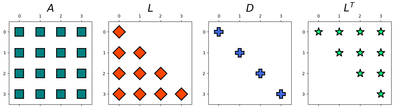
Let $A = [\begin{array}{cccc} 7 & 3 & - 1 & 2 \\ 3 & 8 & 1 & - 4 \\ - 1 & 1 & 4 & - 1 \\ 2 & - 4 & - 1 & 6 \end{array}]$ and $b = [\begin{matrix} 18 \\ 6 \\ 9 \\ 15 \end{matrix}]$ . Then, this linear system can be also expressed as follows,

\begin{array}{r} A x = (L D L^{T}) x = L (D (L^{T} x)) = b . \end{array}

We have,

A = np.array([ [7, 3, -1, 2], [3, 8, 1, -4], [-1, 1, 4, -1], [2, -4, -1, 6] ])
b = np.array([[18],[ 6],[ 9],[15]])
L, D = myLDL(A)
display(Latex(r'L ='), Matrix(np.round(L, 2)))
display(Latex(r'D ='), Matrix(np.round(D, 2)))

L =

\begin{array}{r} [\begin{array}{c} 1.0 & 0 & 0 & 0 \\ 0.43 & 1.0 & 0 & 0 \\ - 0.14 & 0.21 & 1.0 & 0 \\ 0.29 & - 0.72 & 0.09 & 1.0 \end{array}] \end{array}

D =

\begin{array}{r} [\begin{array}{c} 7.0 & 0 & 0 & 0 \\ 0 & 6.71 & 0 & 0 \\ 0 & 0 & 3.55 & 0 \\ 0 & 0 & 0 & 1.89 \end{array}] \end{array}

Now we can solve the following linear systems instead $ ${\begin{cases} L z = b, \\ D y = z, \\ B^{T} x = y . \end{cases}$ $

hd.matrix_decomp_fig(mats = [A, L, D, L.T], labels = ['$A$', '$L$', '$D$','$L^T$'], nrows=1, ncols=4, figsize=(16, 4))

../_images/45ab29e3e653ac4b5015b19cca0e58c4e9269c4a1a4d6e5f5344c33eab905175.png

# solving for z
z = np.linalg.solve(L, b)
display(Latex(r'z ='), Matrix(np.round(z, 2)))

z =

\begin{array}{r} [\begin{array}{c} 18.0 \\ - 1.71 \\ 11.94 \\ 7.54 \end{array}] \end{array}

# solving y
y = np.linalg.solve(D, z)
display(Latex(r'y ='), Matrix(np.round(y, 2)))

y =

\begin{array}{r} [\begin{array}{c} 2.57 \\ - 0.26 \\ 3.36 \\ 4.0 \end{array}] \end{array}

# solving for x
x = np.linalg.solve(L.T, y)
display(Latex(r'x ='), Matrix(np.round(x, 2)))

x =

\begin{array}{r} [\begin{array}{c} 1.0 \\ 2.0 \\ 3.0 \\ 4.0 \end{array}] \end{array}

Let’s now solve the linear system directly and compare the results.

x_new = linalg.solve(A, b)
display(Latex(r'x ='), Matrix(np.round(x_new, 2)))

x =

\begin{array}{r} [\begin{array}{c} 1.0 \\ 2.0 \\ 3.0 \\ 4.0 \end{array}] \end{array}

LDL decomposition

Contents

7.4. LDL decomposition#

7.4.1. Solving Linear systems using LDL decomposition#